A batch of cells arrives at the lab. Before committing them to a weeks-long aging campaign, you run a quick characterization check to screen for outliers and confirm consistency. The question is: do you measure AC internal resistance or DC internal resistance?
Short answer: both, but for different reasons. ACIR gives you a fast, SOC-insensitive check of ohmic health (bad welds, contact issues, electrolyte fill problems), though the frequency you choose determines how much charge transfer leaks in. DCIR with a defined pulse catches everything ACIR catches plus charge transfer kinetics and solid-state diffusion, the components that degrade during storage or cycling. Running both takes under a minute per cell. When they diverge, that tells you more than either number alone.
The rest of this post uses simulations run by Ionworks using PyBaMM to show exactly what each measurement sees, why they give different answers, and how to choose for a given scenario.
Two measurements, two answers
DCIR applies a current pulse (typically 1C to 3C for a few seconds) and divides the voltage drop by the current:
R_DCIR = ΔV / I
ACIR extracts the impedance magnitude |Z| at a single frequency, usually 1 kHz, from an EIS measurement or an AC milliohm meter.
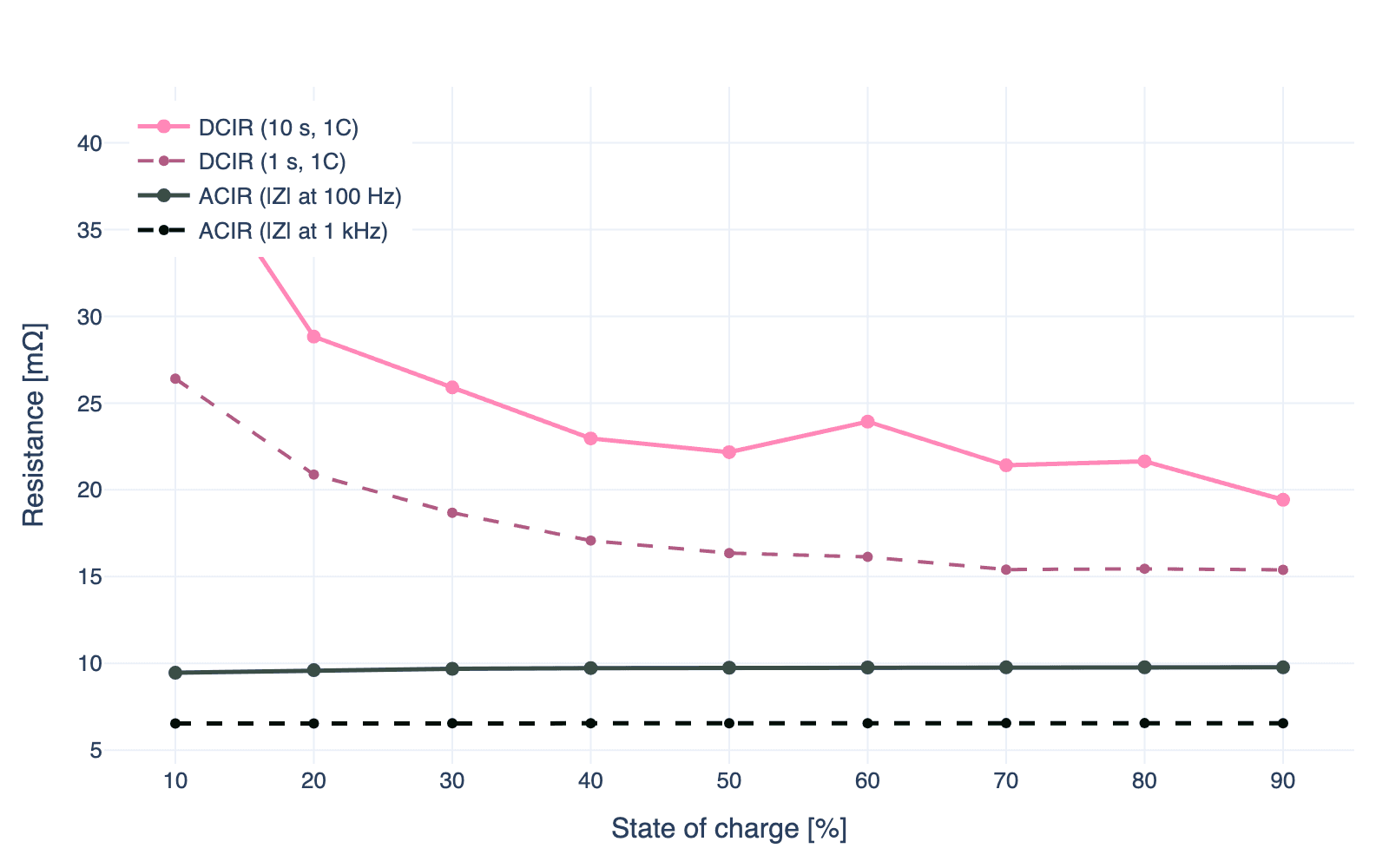
Both are reported as "internal resistance." But on the same cell at the same SOC, DCIR (10 s pulse) returns around 22 mΩ while ACIR at 1 kHz returns 6.6 mΩ and ACIR at 100 Hz returns 9.8 mΩ. Three different numbers from the same cell. If you are screening a batch for consistency, the metric you pick determines which cells you flag.
What each measurement sees
DCIR captures everything between the open-circuit voltage and the loaded terminal voltage: ohmic resistance in the current collectors, tabs, and electrolyte; charge transfer resistance at both electrode interfaces; and, depending on pulse duration, solid-state diffusion within the active material particles. Longer pulses capture more diffusion. A 1 s pulse primarily sees ohmic and charge transfer effects. A 10 s pulse adds a significant diffusion component.
ACIR extracts impedance at a chosen frequency. At 1 kHz, the double-layer capacitance at the electrode-electrolyte interface presents a low-impedance path that shunts current around the faradaic reaction. ACIR at 1 kHz measures the ohmic resistance of the cell (current collectors, tabs, electrolyte, separator, contact resistance) and almost nothing else. At lower frequencies, the capacitive bypass becomes less effective and some charge transfer resistance leaks into the measurement. ACIR at 100 Hz is noticeably higher than at 1 kHz for this reason.
This is not an approximation. It is the physics: under DC load, the capacitor fully charges and blocks current, forcing it through the charge transfer pathway. Under a high-frequency AC signal, the capacitor never fully charges, so most current takes the capacitive shortcut. The higher the frequency, the more current bypasses the faradaic path. The result is that ACIR is always less than DCIR, and ACIR decreases as frequency increases. This holds regardless of cell chemistry, SOC, or temperature.
Simulating both on the same cell
We simulate both measurements on a virtual LG M50 (NMC811/graphite, 5 Ah) using the O'Regan 2022 parameter set, which has experimentally fitted Arrhenius dependences for exchange current density and solid-state diffusivity. The model is PyBaMM's SPMe with surface form: 'differential', which resolves the double-layer capacitor as an explicit state variable. This is critical for getting the ACIR/DCIR split right. We also include an explicit 2 mΩ contact resistance, representing tab and connection losses.
DCIR protocol: 5 s rest, 10 s discharge at 1C, 5 s rest.
ACIR protocol: EIS sweep from 1 mHz to 10 kHz. We extract |Z| at 1 kHz and 100 Hz. The wide frequency range lets us visualize the full Nyquist plot (ohmic intercept, charge transfer semicircle, diffusion tail) and shows how the choice of frequency changes what ACIR captures.
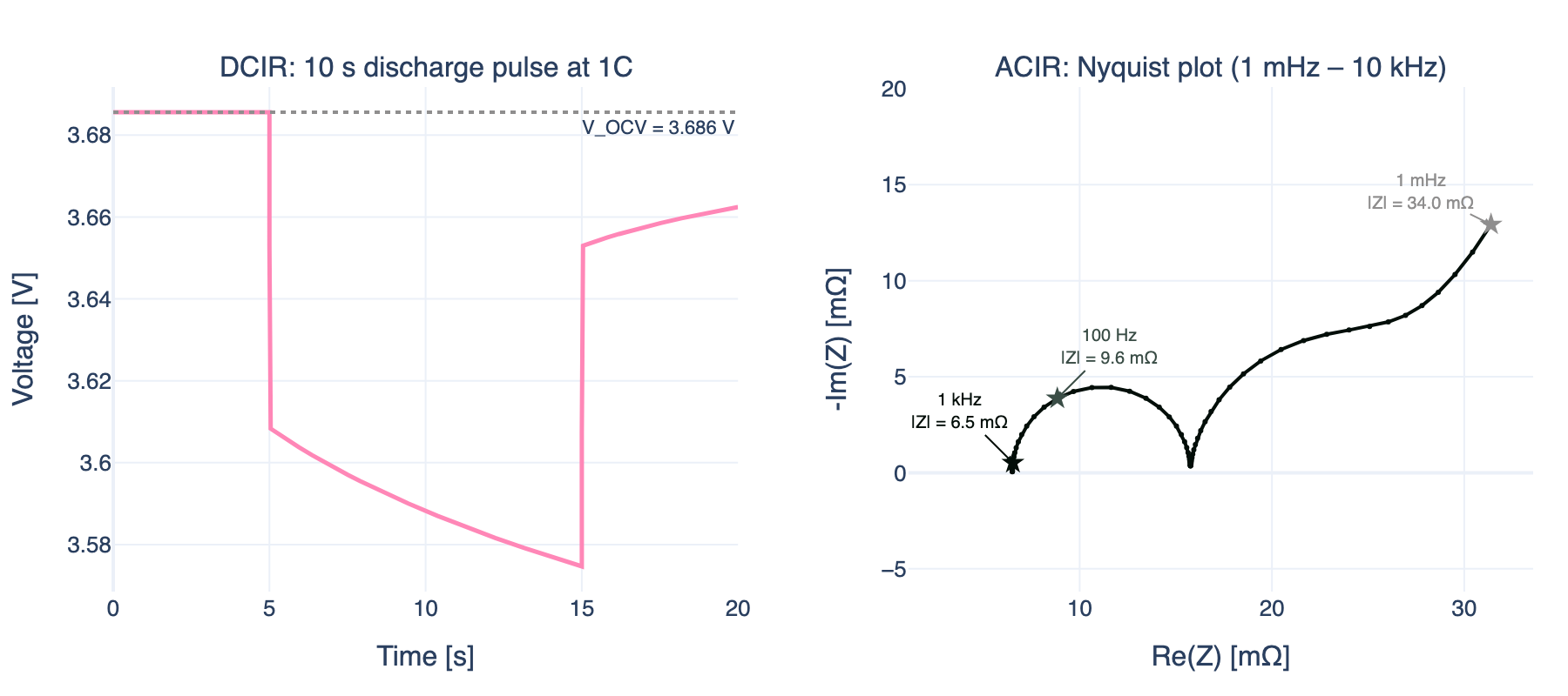
The Nyquist plot makes the difference visual. The 1 kHz point sits at the leftmost edge of the spectrum, before any of the slower processes contribute. The DC pulse sits at the far right. It sees everything.
What makes up the DCIR
The DCIR number is not a single physical quantity. It is the sum of several transport processes that activate at different timescales during the pulse. PyBaMM tracks each overpotential component separately, so we can extract the resistance contribution from each and see how they stack up.
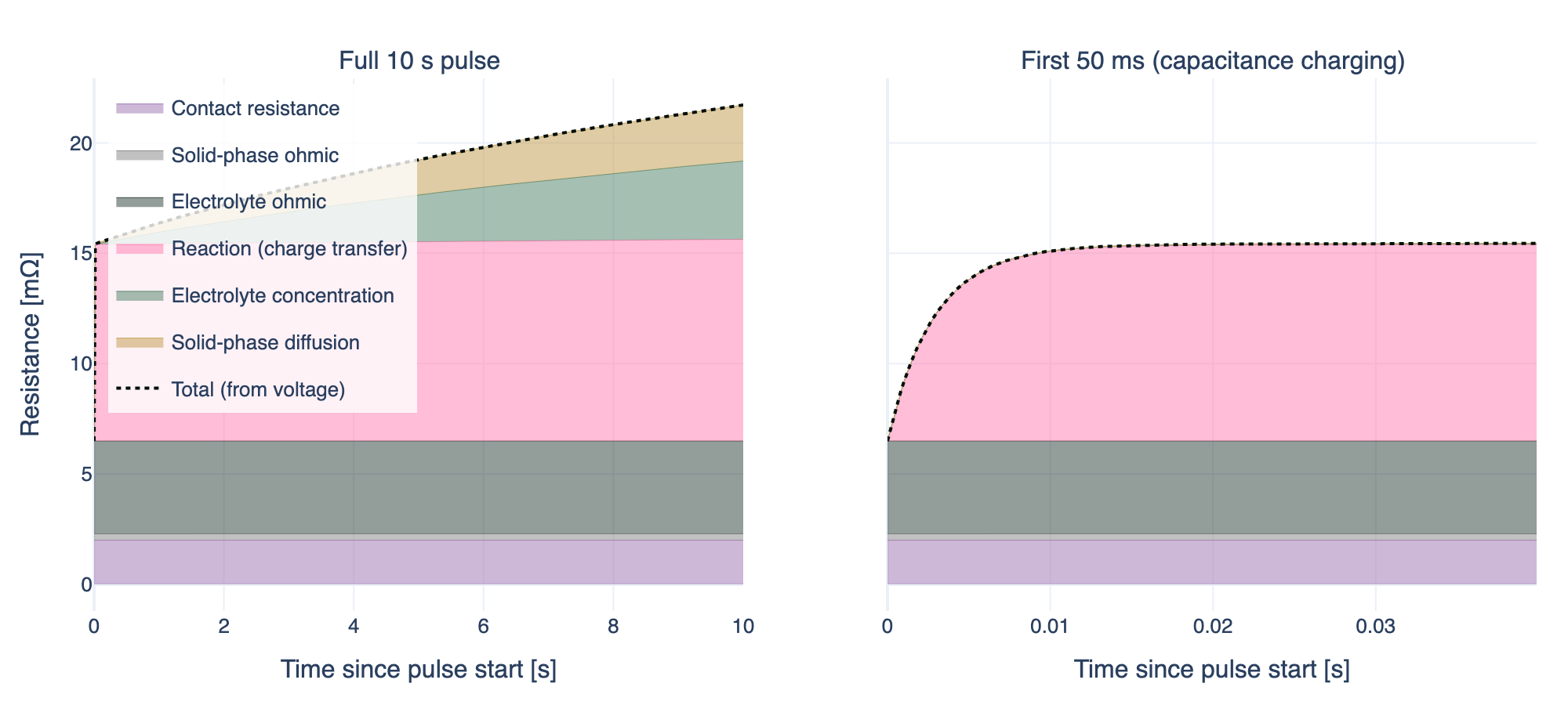
The stacked areas show what the pulse accumulates over time:
- Contact resistance, solid-phase ohmic, and electrolyte ohmic appear instantly. These are the purely resistive components: tab and weld connections, electrode bulk conductivity, and ion transport through the electrolyte. Together they make up the ohmic baseline, close to the ACIR value at 1 kHz.
- Reaction (charge transfer) resistance dominates. The zoom panel shows it ramping up over the first ~50 ms as the double-layer capacitor charges. Before the capacitor is fully charged, some current flows through it instead of through the faradaic pathway, reducing the apparent resistance. This is exactly the mechanism that makes ACIR lower: the 1 kHz signal never lets the capacitor fully charge.
- Electrolyte concentration and solid-phase diffusion grow steadily over the full 10 s. These are the components that make a 10 s DCIR larger than a 1 s DCIR. Since you can sample the voltage at both 1 s and 10 s from the same pulse, a single test gives you both values at no extra cost.
For a pre-test screen, this decomposition matters. If you only measure ACIR at 1 kHz, you see the ohmic pathway and nothing else. A cell with cracked particles (degraded diffusion) or poisoned surface films (increased charge transfer resistance) would return the same ACIR as a fresh cell. ACIR at 100 Hz picks up some charge transfer contribution, so it has slightly more diagnostic reach, but still misses the diffusion component entirely.
What frequency means for ACIR
ACIR is not a single number. It depends on the excitation frequency, and the relationship is not linear. To see why, we plot ACIR |Z|(f) from the EIS sweep alongside DCIR ΔV/I sampled at time t and mapped to an equivalent frequency f = 1/(2πt). This puts both measurements on a shared axis so we can compare them directly.
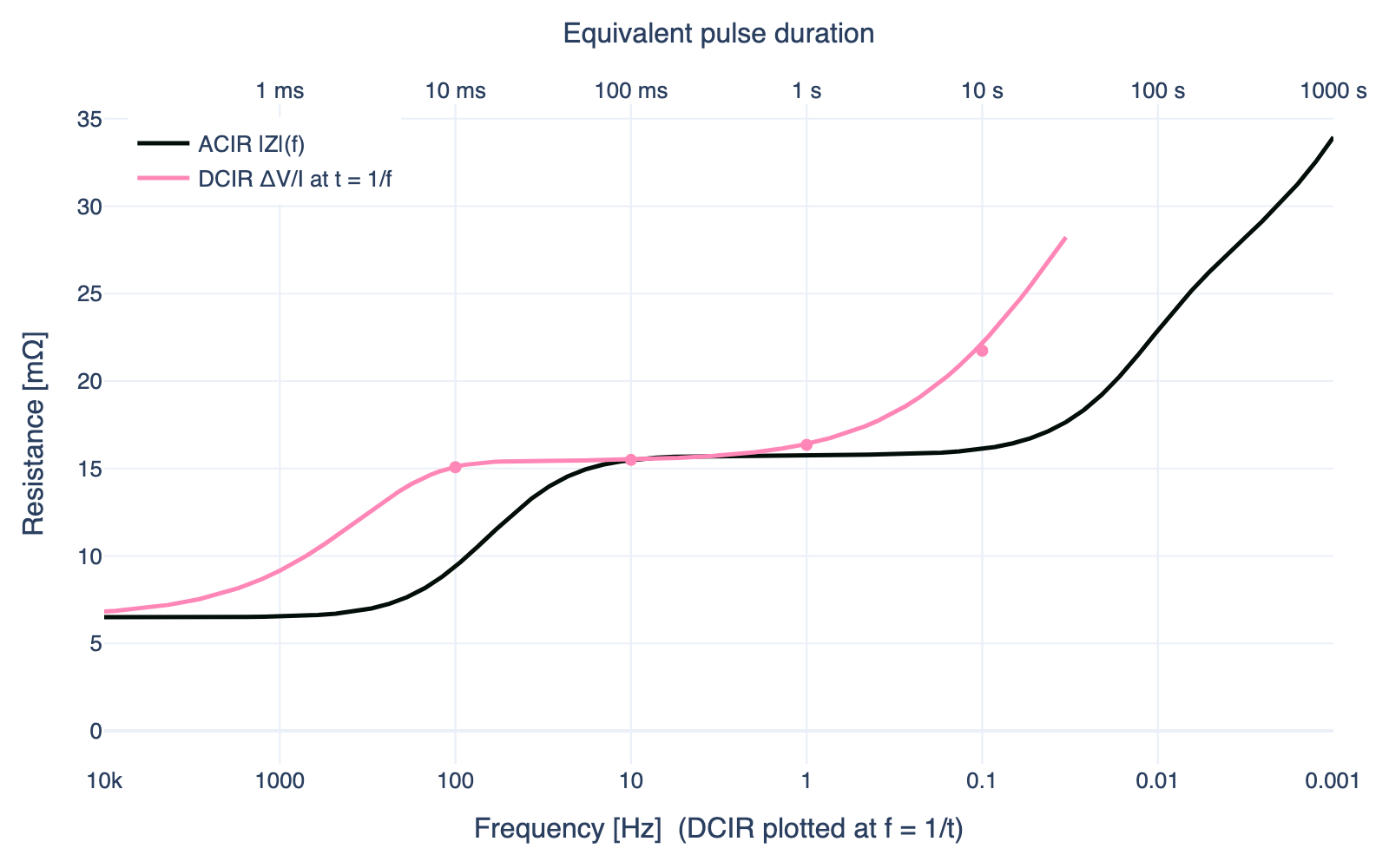
Both curves rise from left to right as slower processes come in: flat at high frequencies where only ohmic resistance contributes, steepening through charge transfer, then climbing where diffusion dominates. The two curves nearly overlap across the full frequency range, confirming that ACIR and DCIR are probing the same underlying impedance — the difference between the two measurements is primarily one of timescale, not of kind. (The 2π in the mapping comes from the relationship between ordinary frequency and angular frequency. The simpler mapping f = 1/t overstates the gap between the curves, but the physics is the same either way.)
Where the curves do separate slightly, the gap reflects the broadband nature of the DC pulse. A sinusoid at frequency f probes one timescale in isolation. A step function contains all frequencies simultaneously, so even at short times the pulse includes contributions from slower processes that have begun to activate. This makes DCIR slightly higher than ACIR at the same equivalent frequency, but the effect is small.
This matters for instrument selection and cross-site comparisons. Two labs measuring "ACIR" at different frequencies will get different numbers from identical cells. If your incoming inspection uses an AC milliohm meter at 1 kHz and your supplier's datasheet quotes impedance at 120 Hz, the values are not comparable without understanding what each frequency captures. However, the close agreement between the correctly scaled curves means you can approximate DCIR from an impedance spectrum by reading |Z| at f = 1/(2πt) for the pulse duration of interest — a useful shortcut when full DCIR testing is not practical.
How SOC affects each measurement
When screening a batch, cells may arrive at slightly different states of charge. How much does that matter for each metric?
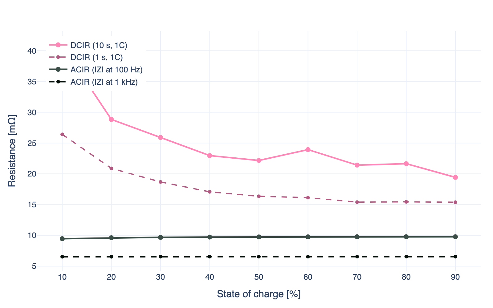
- DCIR varies significantly with SOC; ACIR barely moves. DCIR (10 s) swings across the SOC range while both ACIR traces stay nearly flat. The ohmic resistance does not change with lithium intercalation state. The SOC-dependent components (charge transfer and diffusion) are invisible to the 1 kHz signal and only partially visible at 100 Hz.
- The gap between ACIR frequencies is consistent across SOC. ACIR at 100 Hz sits above ACIR at 1 kHz by a roughly constant offset, reflecting the charge transfer contribution that leaks through at the lower frequency. Neither trace shows the SOC sensitivity that DCIR does.
- Pulse duration matters for DCIR. The 1 s pulse gives consistently lower values than 10 s because it has less time to accumulate the diffusion contribution.
The practical implication for screening: ACIR at either frequency is insensitive to SOC variation in the batch. If cells arrive at different charge levels, ACIR still gives you a clean comparison of ohmic health. DCIR requires that you either bring cells to the same SOC first or accept that SOC spread will broaden your distribution and mask real defects.
How temperature widens the gap
Lab temperature is usually controlled. Warehouse temperature is not. If cells arrive in winter from an unheated shipping container, the resistance you measure at 10°C looks very different from the same cell at 25°C. How much does that matter for each metric?
We simulate both measurements across a temperature range. The O'Regan 2022 parameter set has experimentally fitted Arrhenius dependences for the exchange current density and solid-state diffusivity, so the temperature effects on kinetics and transport are physically grounded.
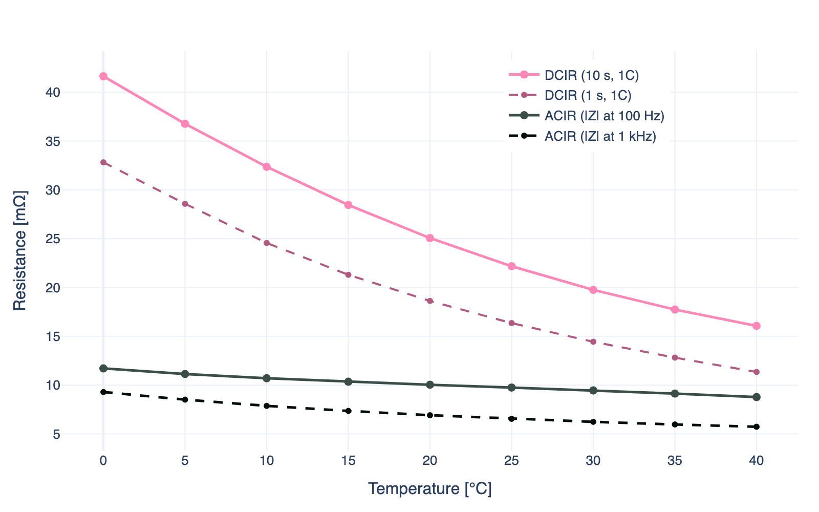
ACIR at 1 kHz increases modestly at low temperatures. Electrolyte conductivity drops with temperature, raising the ohmic resistance, but the effect is gradual. ACIR at 100 Hz rises more steeply because the charge transfer component it captures also slows with temperature. DCIR increases the most. The exchange current density and solid-state diffusivity both follow Arrhenius kinetics: they drop exponentially as temperature falls, so the charge transfer and diffusion contributions to DCIR grow fast.
At 25°C the gap between all four metrics is already visible. At 10°C it widens substantially. At 0°C the DCIR is dominated by sluggish kinetics and diffusion, while ACIR at 1 kHz still reflects mostly the ohmic pathway. ACIR at 100 Hz sits between the two, confirming that it captures a temperature-sensitive kinetic component that 1 kHz misses.
For screening, this means: if you measure DCIR at goods-in without controlling or recording temperature, you cannot separate a cold cell from a degraded cell. ACIR at 1 kHz is the least sensitive to temperature because it only sees the ohmic component. For incoming inspection in environments without tight temperature control, ACIR gives a cleaner signal. If you do measure DCIR, always log the temperature and compare cells measured at the same conditions.
Which parameters each measurement catches
The SOC and temperature sweeps show how operating conditions affect the gap between ACIR and DCIR. But when deciding what to measure in a pre-test check, you also need to know what defects each metric can detect. We sweep six material parameters independently at 50% SOC, showing DCIR (1 s and 10 s) alongside ACIR (100 Hz and 1 kHz):
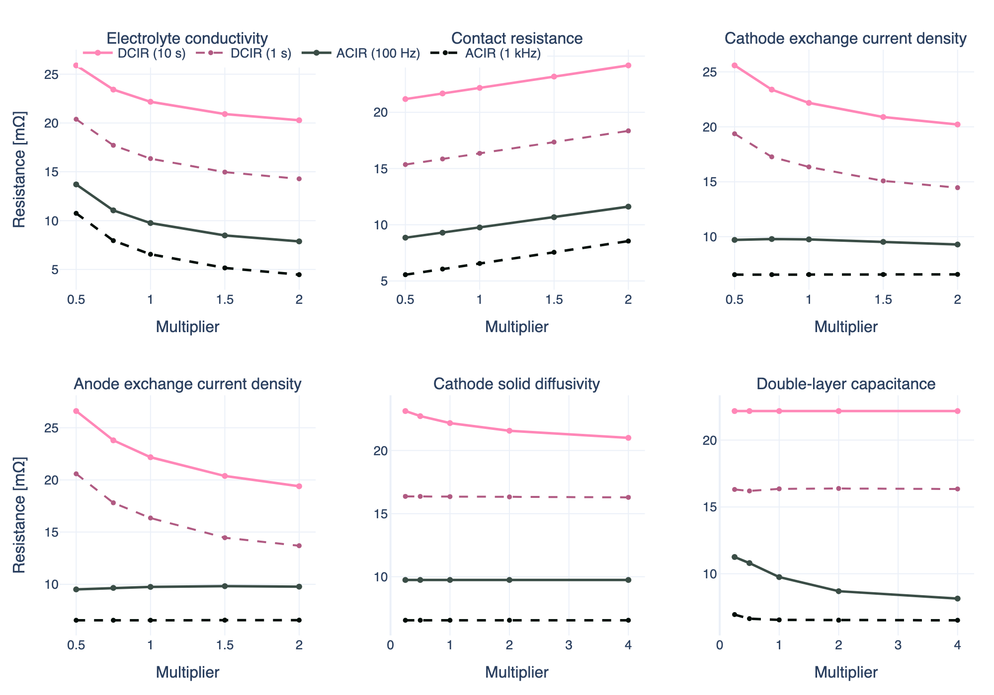
Electrolyte conductivity and contact resistance affect all four metrics. Tab corrosion, dried-out electrolyte, and weld defects show up regardless of which resistance you measure.
Charge transfer kinetics (exchange current density at either electrode) shift both DCIR values clearly. ACIR at 1 kHz is unaffected, but ACIR at 100 Hz picks up a small sensitivity. At 100 Hz, enough of the charge transfer arc leaks through the capacitive bypass to register changes in surface kinetics. This is one practical reason to measure ACIR at a frequency below 1 kHz: you gain partial visibility into electrode kinetics without the SOC sensitivity that comes with a full DC pulse. The cathode and anode exchange current densities have different magnitudes of effect, which matters if you are trying to localize degradation to one electrode.
Solid-state diffusivity in the positive electrode affects 10 s DCIR more than 1 s DCIR, and has no effect on either ACIR frequency. This is the parameter that separates the two pulse durations: a 1 s pulse barely samples the diffusion contribution, while a 10 s pulse accumulates it. Particle cracking and loss of active material show up more clearly in the longer pulse.
Double-layer capacitance has a subtle but real effect on 1 s DCIR. A larger capacitance means the capacitor takes longer to charge, so the apparent charge transfer resistance is still ramping up when the 1 s measurement window closes. At 10 s the capacitor is fully charged and the effect vanishes. ACIR at 100 Hz also shows some sensitivity here: the capacitance determines how effectively the AC signal bypasses the faradaic pathway at that frequency.
If your pre-test check targets manufacturing defects in the ohmic pathway (bad welds, contact issues, electrolyte fill problems), ACIR at 1 kHz is sufficient and much faster. If you want partial kinetic visibility without SOC sensitivity, ACIR at 100 Hz is a good middle ground. If you need to catch transport degradation (from storage, shipping damage, or prior cycling), you need DCIR. Running both 1 s and 10 s pulses adds a further diagnostic dimension: a cell where 10 s DCIR rises but 1 s DCIR stays flat has a diffusion problem, not a kinetic one.
Choosing your pre-test check
| Scenario | Recommended | Why |
|---|---|---|
| Incoming inspection at goods-in | ACIR (1 kHz) | Fast, no SOC control needed, catches assembly defects |
| Pre-aging baseline for a test matrix | DCIR (defined pulse) | Captures charge transfer and diffusion baseline for tracking changes |
| Screening after storage or transport | Both | ACIR for ohmic damage; DCIR for kinetic or transport degradation |
| SOC not well controlled in the batch | ACIR (either frequency) | Insensitive to SOC variation, cleaner outlier detection |
| Partial kinetic check without SOC sensitivity | ACIR (100 Hz) | Picks up some charge transfer without the SOC dependence of DCIR |
| Diagnosing a flagged cell | Full EIS | Separates ohmic, charge transfer, and diffusion quantitatively |
| BMS resistance parameterization | DCIR at target C-rate and pulse duration | BMS operates in the DC domain |
The measurements are complementary. Running ACIR at two frequencies plus a 10 s DCIR pulse takes under a minute and gives you a layered view of cell health. ACIR at 1 kHz covers the ohmic pathway. Drop to 100 Hz and you pick up partial kinetic information. The 10 s pulse gives you both DCIR values for free: sample the voltage at 1 s and again at 10 s from the same pulse to separate kinetic and diffusion contributions. The diagnostic value is often in the gaps between metrics, not in any single number.
Knowing which resistance to measure, and what it actually tells you, is the difference between a pre-test check that catches problems and one that misses them. Ionworks Studio simulates ACIR at any frequency and DCIR at any pulse duration from the same cell model: define the protocol once, run it in PyBaMM, and compare directly against measured data from any cycler brand. Book a demo to see how teams build pre-test characterization workflows that transfer across instruments and chemistries.
Frequently asked questions
Continue reading