Battery parameter estimation is the work that sits between raw test data and a simulation you can trust. Every battery model needs a parameter set, and the quality of that set decides whether a simulation informs an engineering decision or misleads one. For most R&D teams, building and validating parameter sets is the slowest and least repeatable step in the modeling workflow.
Why parameter estimation is the bottleneck
A cycling test produces voltage, current, and temperature traces. A physics-based simulation requires dozens of transport, kinetic, geometric, and thermodynamic inputs. Parameter estimation is the gap between those two states.
The difficulty scales with model fidelity. An equivalent circuit model (ECM) might need a handful of resistance and capacitance values fitted to pulse data. A full electrochemical model, like the Doyle-Fuller-Newman (DFN) formulation, can require 35 or more parameters drawn from teardown, half-cell, impedance, and pulse experiments, as demonstrated by Chen et al. 2020 for a commercial 21700 cell.
A solver can run in seconds. Assembling a defensible parameter set often takes weeks. That asymmetry is where teams lose time, introduce error, and break reproducibility.
Three model classes, three data burdens
The data burden for battery model parameterization depends on the model class. Framing estimation around three tiers helps teams plan test campaigns and set expectations for what a given model can and cannot resolve.
Equivalent circuit models (ECM)
Equivalent circuit models represent cell behavior with resistors, capacitors, and voltage sources. The canonical first-order Thévenin form uses a state-of-charge dependent open-circuit voltage in series with an ohmic resistance and one or more RC pairs.
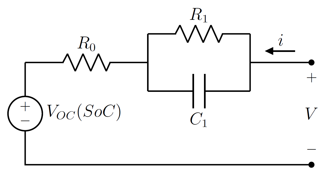
ECMs are purely empirical. They are fitted directly to full-cell current and voltage data and do not simulate any internal electrochemical process. Their strengths are speed, simplicity, and compatibility with BMS environments where state estimation and real-time control matter more than internal physics. The tradeoff is that fitted parameters carry limited physical meaning, predictive accuracy is bounded by interpolation inside the training data, and the model cannot distinguish between positive and negative electrode behavior.
ECM fitting needs time-series current and voltage data from operating conditions that match the intended application window. A pulse discharge at 25°C will not produce a parameter set that works for fast charge at 0°C.
Lumped physics-based models (SPM, SPMe)
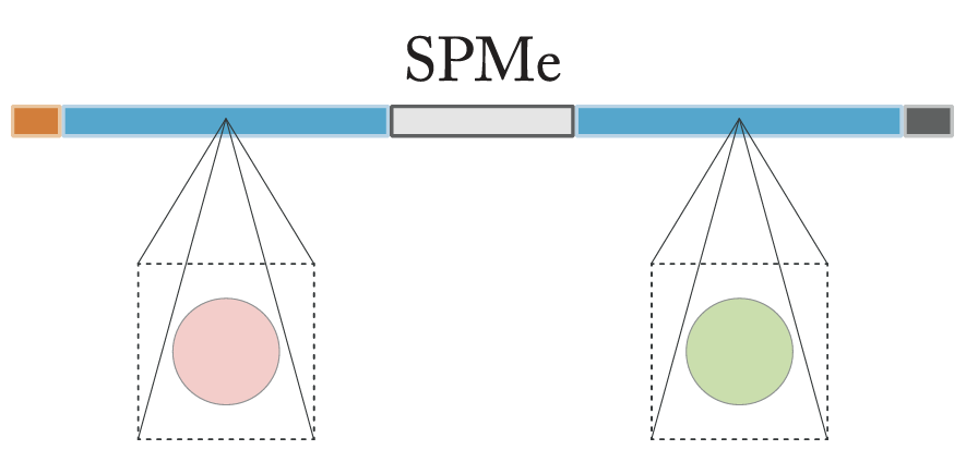
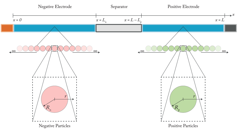
Lumped physics-based models capture intercalation kinetics and solid-phase diffusion in each electrode, but simplify the spatial variation across the cell by assuming uniformity through the electrode thickness. The Single Particle Model (SPM) represents each electrode as a single representative particle. The SPMe variant adds electrolyte dynamics on top of that reduction.
Lumped physics-based models sit between ECMs and full physics. They simulate electrode-specific state of charge, overpotentials, and internal heat generation without requiring full teardown data. That makes them useful for diagnosing cell imbalances or degradation precursors when a DFN campaign is out of budget. The limitations are real: they rely on fitted OCV curves for each electrode, they cannot resolve electrolyte gradients or electrode heterogeneity, and they can miss local effects like lithium plating or electrolyte depletion.
The key thing to understand about "lumped" parameterization is what it does and does not resolve. Lumping does not mean fitting fewer individual parameters. It means fitting the dimensionless or dimensional groups that the full-cell response is actually sensitive to, instead of trying to recover each underlying physical quantity separately. Full-cell voltage and current data cannot tell you the particle radius R and the solid-phase diffusivity D independently, because they only enter the cell-level response through the diffusion timescale τ = R²/D. In the same way, electrode area A, coating thickness L, active material volume fraction ε, and maximum lithium concentration c_max are not separately identifiable from full-cell cycling — only the lumped electrode capacity Q = A·L·F·ε·c_max/3600 (in Ah) shows up in the data. A lumped parameterization fits τ and Q directly and stops there. That is why teardown is not required: the model is honest about what the experiment can resolve.
SPM and SPMe parameterization typically needs full-cell OCV data, rate capability tests across multiple C-rates, and HPPC or pulse data for the lumped diffusion timescales and reaction rate groups. SPMe parameterization adds an analogous lumped treatment of electrolyte transport and usually requires richer fitting but remains tractable from standard full-cell experiments.
Full physics-based models (DFN)
Full physics-based models solve coupled partial differential equations for conservation of mass, charge, and energy across both electrodes, the separator, and the electrolyte. The DFN (pseudo-2D) formulation resolves solid-phase diffusion, electrolyte transport, and reaction kinetics across the cell thickness.
These models provide the highest fidelity available for cell-level simulation. They can capture spatial heterogeneity, electrolyte depletion, overpotential distributions, and the precursors to failure modes like lithium plating at high rate or low temperature. They are also the natural home for degradation mechanism modeling, where SEI growth, particle cracking, and loss of active material couple back into the electrochemistry.
The cost is parameter intensity. DFN parameter estimation requires teardown measurements, half-cell experiments, stoichiometric window identification, kinetic and diffusion parameters, and thermal characterization. Chen et al. 2020 documented an experimental workflow that includes GITT, EIS, three-electrode full-cell configurations, and current-pulse analysis (Sand equation) to populate a 35-parameter dataset for a P2D model. Parameter identification is complex, computational cost is an order of magnitude above lumped models, and the data requirement is often a barrier in early-stage projects.
What battery parameter estimation actually means
Battery parameter estimation means building a complete, usable parameter set for a chosen model class. Curve fitting is one step in that process. The work also includes selecting which parameters to fit versus fix, choosing appropriate test data, applying physical constraints, and validating the resulting set against independent experiments.
A voltage curve that looks correct is not proof that the underlying parameters are correct. Laue et al. 2021 showed that P2D models are prone to unidentifiability: different parameter combinations can produce similar voltage outputs, and fitting to a narrow dataset can mask physically unreasonable values.
Battery model calibration, battery parameterization, and electrochemical model parameter estimation refer to the same problem. The goal is a parameter set that is physically plausible, identifiable from the available data, and validated on conditions outside the fitting set.
A step-by-step view of what each model needs
The clearest way to frame a parameterization campaign is to walk through the experimental steps in order. Each step constrains a specific set of parameters, and later steps depend on the outputs of earlier ones.
DFN parameterization
A typical DFN workflow splits into five steps, moving from electrode-level measurements up to full-cell dynamics and thermal behavior.
| Step | Data required | Parameters fitted |
|---|---|---|
| 1 | Half-cell OCV curves | Electrode OCV curves |
| 2 | Full-cell OCV curve | Electrode capacities; initial particle concentrations |
| 3 | Cell teardown | Geometric parameters (electrode dimensions, particle sizes, porosities, active material volume fraction); maximum concentrations |
| 4 | Full-cell rate capability and pulse test (voltage) | Particle diffusivities (T, SOC); exchange-current densities (T, SOC); electrolyte properties (diffusivity, conductivity, T, concentration) |
| 5 | Full-cell rate capability and pulse test (temperature) | Thermal capacity; heat transfer coefficients (core and surface) |
Pulse tests here can be HPPC, GITT, or any DCIR protocol at multiple states of charge. Diffusivities, exchange-current densities, and electrolyte properties are all functions of temperature and, in most cases, concentration or SOC. Fitting those as constants collapses physics the model was built to capture.
Lumped physics-based parameterization
SPM and SPMe parameterization is lighter. Teardown and half-cell data are replaced with a single full-cell OCV characterization, and transport parameters are fitted as lumped groups rather than resolved at the particle and electrolyte level.
| Step | Data required | Parameters fitted |
|---|---|---|
| 1 | Full-cell OCV curve | Electrode OCV curves; lumped electrode capacities Q = A·L·F·ε·c_max/3600; initial stoichiometries |
| 2 | Full-cell rate capability and pulse test (voltage) | Lumped solid diffusion timescales τ = R²/D (T, SOC); lumped reaction rate groups (T, SOC) |
| 3 | Full-cell rate capability and pulse test (temperature) | Thermal capacity; heat transfer coefficients |
The tradeoff is visible in step 1. Lumped models back out electrode OCV contributions and lumped capacities from full-cell data rather than measuring A, L, ε, and c_max independently against lithium metal. That is cheaper and faster, and it also means the identifiability of those curves depends on the quality of the fit. The upside is that the parameters that are fitted, τ and Q, are exactly the groups the full-cell experiment can resolve — there is no pretense of recovering quantities the data does not constrain.
ECM parameterization
ECM parameterization reduces to two steps built around dynamic full-cell data.
| Step | Data required | Parameters fitted |
|---|---|---|
| 1 | Full-cell rate capability and pulse test or drive cycle (voltage) | Open-circuit voltage (SOC); series resistance (SOC, current, T); RC pairs (SOC, current, T) |
| 2 | Full-cell rate capability and pulse test or drive cycle (temperature) | Thermal model parameters |
If the ECM will be used to predict dynamic duty cycles, the fitting data should include dynamic current profiles. Coverage of the SOC, current, and temperature operating window matters more than the total volume of data.
Data requirements at a glance
The same content, collapsed into a single matrix, shows where the cost lives.
| Data required | DFN | Lumped (SPM/SPMe) | ECM |
|---|---|---|---|
| Full-cell rate capability and pulse test (voltage) | ✓ | ✓ | ✓ |
| Full-cell rate capability and pulse test (temperature) | ✓ | ✓ | ✓ |
| Full-cell OCV curve | ✓ | ✓ | |
| Cell teardown | ✓ | ||
| Half-cell OCV curves | ✓ |
The thermal test is only required for temperature predictions. The dynamic voltage test is the common foundation across all three model classes. Everything above it, OCV, teardown, half-cell, exists to resolve the ambiguities that dynamic data alone cannot fix.
Why parameter sets fail
Parameter sets fail for specific, diagnosable reasons. Understanding these failure modes helps teams build estimation workflows that produce trustworthy results.
Weak observability. When too many unknowns are fitted from too few test modalities, the optimization finds a combination that matches the data without being physically correct. A different combination might fit equally well. This is the identifiability problem documented across the electrochemical modeling literature.
Mixed provenance. Teams often assemble parameter sets from multiple sources: some values from literature, some from in-house tests, some inherited from a previous project. When those sources refer to different cells, conditions, or measurement setups, the resulting set may be internally inconsistent.
Overfitting. Fitting to a narrow dataset (one temperature, one C-rate, one SOC window) can produce a parameter set that looks excellent on the training data and fails on anything else. Overfitting is especially likely with high-dimensional models where many parameters interact.
Reused validation data. If the data used to validate a parameter set is the same data used to fit it, the validation is meaningless. Held-out experiments, ideally at different operating conditions, are required for a credible check.
How validated parameter sets are built
A defensible battery parameter estimation workflow follows a consistent sequence. Each step produces an artifact that the next step depends on.
- Choose the model class. The model determines which parameters are needed, which can be measured directly, and which must be fitted. ECM, SPM, SPMe, and DFN each imply a different estimation program.
- Gather the required data. Design and execute the test campaign for the chosen model class. Structure the resulting measurements with clear metadata: cell identity, test conditions, equipment, timestamps.
- Fit parameters. Use optimization or direct extraction to estimate unknown parameters. Apply physical bounds and fix parameters that are directly measured or well-established. PyBaMM exposes the forward model and parameter sensitivities a fitter needs, but assembling the optimization, identifiability checks, and bookkeeping around it is left to the user.
- Check plausibility. Compare fitted values against literature ranges and physical expectations. A diffusion coefficient that differs from published values by three orders of magnitude warrants investigation, regardless of fit quality.
- Validate. Run the parameterized model against held-out experiments. Validation data should cover operating conditions that were not part of the fitting set.
- Freeze. Lock the validated parameter set with a version identifier and a record of its provenance: which data informed each parameter, which assumptions were applied, which validation experiments confirmed the result.
PyBaMM and the model ladder
Many battery simulation parameter estimation queries reference PyBaMM model names directly. PyBaMM implements the standard model ladder for lithium-ion cells, and its documentation provides comparison notebooks and parameterization workflows for each class.
| PyBaMM model | Model class | Typical estimation complexity |
|---|---|---|
| ECM | Equivalent circuit | Low: pulse fitting, RC time constants |
| SPM | Lumped physics-based | Moderate: OCV, rate capability, pulse data |
| SPMe | Lumped physics-based | Moderate to high: adds electrolyte transport |
| DFN | Full physics-based | High: electrode-resolved data, EIS, teardown |
PyBaMM provides Parameter Values objects, BPX file support, and the forward-model and sensitivity primitives a fitter can call into. It does not provide a turnkey parameter estimation workflow — wiring up the optimizer, identifiability checks, and validation loop remains the user's job. What it also does not handle is the organizational layer: tracking which measurements fed a given parameter set, connecting cell identities to test data, versioning parameterized models, and keeping previous fits reproducible months later.
From one-off fits to a team workflow
One engineer in a notebook can produce a working parameter set. Problems appear when a second engineer needs to reproduce the fit, when a team needs to compare parameter sets across cells or aging states, or when a project picks up six months later and the original analyst has moved on.
Ionworks provides the production layer around PyBaMM for teams that need repeatable, traceable battery model parameterization. A parameterized model in Ionworks bundles a model class, a validated parameter set, and a cell specification into a single artifact. Its provenance records which measurements informed which values, which assumptions were applied, and which validation runs confirmed the result.
Measurement data is treated as structured, first-class objects tied to specific cells and test conditions. Time-series data, checkpoint measurements, and electrochemical characterization results are organized so that downstream fitting workflows reference them directly rather than pointing to filenames on a shared drive.
The same workflow scales across model classes. An ECM fit against pulse and drive-cycle data, an SPMe fit against OCV and rate capability, and a DFN fit against teardown, half-cell, GITT, and EIS data all land in the same system of record. When a team updates an OCV curve or adds a new C-rate test, the parameterized models affected by that change are identifiable through their provenance.
This traceability matters most for battery degradation modeling, where parameter sets evolve over a cell's lifetime. A team studying capacity fade needs to track how parameters shift with aging, and each aging state needs its own validated parameter set tied to specific characterization data.
What better parameterization changes
When a parameter set is validated once and reusable across studies, the time between a test campaign and an engineering recommendation shrinks. When validation runs come from held-out experiments with clear provenance, confidence in simulation-driven decisions rises. When a parameter set built in one lab can be reviewed and extended by another team without reverse-engineering a notebook, collaboration becomes practical across projects and over time.
Ionworks Studio's Train stage orchestrates the full parameterization workflow — from experimental design through fitting, validation, and versioning — without requiring teams to hand-code optimization loops. It combines PyBaMM's physics, fast solvers, and extensible parameter interface with the organizational layer that makes parameterization repeatable: measurement tracking, provenance recording, and model versioning.
Bring a dataset. Leave with a parameterized model. Walk through the full fitting and validation workflow with our team on your own data.
Frequently asked questions
Continue reading