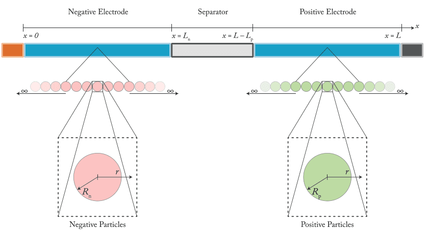
A cell design team and a modelling team are looking at the same electrode and describing it with different numbers. The modeller's parameter file says the positive electrode is 75.6 µm thick with a porosity of 0.335. The process engineer knows what porosity is, but it is not something the line sets directly. That electrode was built to hit a target mass loading of 24 mg/cm² at a press density of 3.19 g/cm³, and those are the two numbers the process team actually controls.
Both descriptions are correct. They describe the same electrode. But neither team can work in the other's variables without recomputing, and the recomputation hides a pair of assumptions (crystallographic density of the active material, and what fraction of the pressed solid is active) that nobody writes down because nobody has to, until suddenly they do.
This is the kind of friction that slows physics-based models down in industry. The model is accurate. The factory is producing cells. The handoff between them leaks information every time it runs.
Same electrode, different vocabularies
Most battery parameter files, including those in the PyBaMM library, store the electrode geometry as thickness and porosity. That is the natural choice for a modeller: both quantities appear directly in the governing equations, and both are measurable on a cross-section.
A cell designer or process engineer works one level up. They specify mass loading (how many grams of active coating per cm² of current collector) and press density (how tightly that coating is compacted after calendering). Mass loading sets the capacity per unit area. Press density sets how close the electrode sits to its theoretical packing limit, and that in turn controls the porosity that the electrolyte has to wick into.
These are related by geometry, but the relationship is not a simple renaming.
porosity                 = 1 - press_density / crystallographic_density
thickness [m]            = mass_loading [g/cm²] / (press_density [g/cm³] * 100)
active vol frac (solid)  = f * press_density / crystallographic_density
where f is the active-material fraction of the pressed solid (the rest is binder and conductive carbon) and crystallographic_density is a chemistry property: roughly 2.2 g/cm³ for graphite, 4.8 g/cm³ for NMC811, 3.6 g/cm³ for LFP.
Four physical inputs the process engineer cares about (mass loading, press density, crystallographic density, and the active fraction of the pressed solid) map cleanly onto the three modeller-facing quantities (thickness, porosity, active material volume fraction). Changing any of the inputs should propagate through every derived quantity that depends on it, consistently.
Linked parameters
Most parameter files in the PyBaMM ecosystem store everything as numbers. You open a JSON file, you see Positive electrode thickness [m]: 7.56e-5, and if you want to ask "what happens if I thin the electrode by 10%," you edit the number. If thinning the electrode should also change the porosity (because the variable you actually adjusted was press density, not thickness) there is no indication of that anywhere in the file.
Linked parameters address this by letting a parameter be a symbolic expression over other parameters. The numeric inputs are the quantities you want to drive the design with. The derived quantities are symbolic. Editing an input propagates through every expression that references it.
Applied to the Chen2020 parameter set, that looks like this:
import pybamm

base = pybamm.ParameterValues("Chen2020")
pv = base.copy()

for electrode in ["negative", "positive"]:
    E = electrode.capitalize()

    # Pick inputs the process engineer thinks in
    pv[f"{E} electrode crystallographic density [g.cm-3]"] = 4.8  # NMC811
    pv[f"{E} electrode press density [g.cm-3]"] = 3.19
    pv[f"{E} electrode mass loading [g.cm-2]"] = 0.0241
    pv[f"{E} electrode active volume fraction of solid"] = 0.665 / (1 - 0.335)

    # Bind them as symbols
    pd = pybamm.Parameter(f"{E} electrode press density [g.cm-3]")
    ml = pybamm.Parameter(f"{E} electrode mass loading [g.cm-2]")
    cd = pybamm.Parameter(f"{E} electrode crystallographic density [g.cm-3]")
    f  = pybamm.Parameter(f"{E} electrode active volume fraction of solid")

    # Rewrite the modeller-facing parameters as symbolic expressions
    pv[f"{E} electrode thickness [m]"]                        = ml / (pd * 100)
    pv[f"{E} electrode porosity"]                             = 1 - pd / cd
    pv[f"{E} electrode active material volume fraction"]      = f * pd / cd
The full recast that we used for the figures in this post is a short Python file that sits on top of any PyBaMM parameter set. At the base point, the recast parameter set evaluates identically to Chen2020: same thickness, same porosity, same active volume fraction. Nothing has changed numerically. What has changed is which inputs you reach for when you want to explore a design.
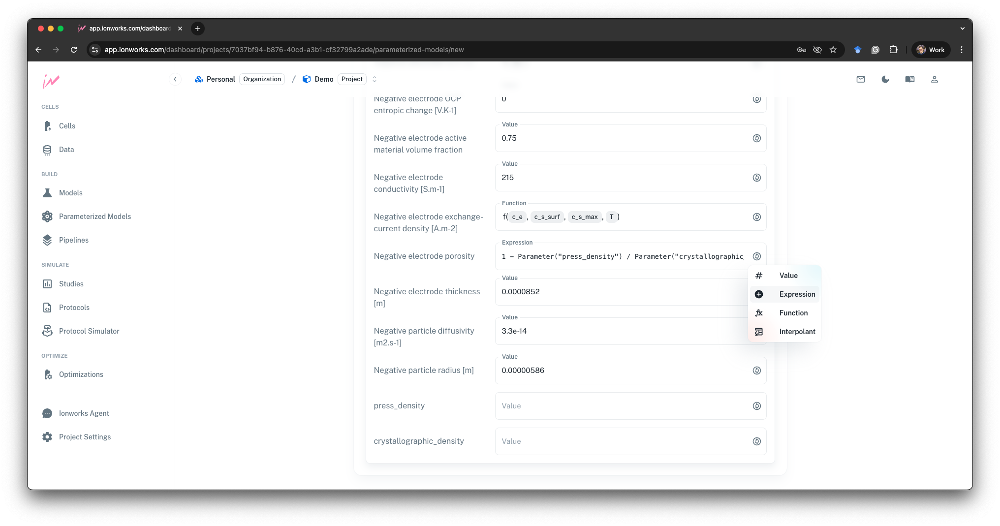
A script is fine for a blog post, but it is the wrong place for this definition to live in a real workflow. If the link between mass loading, press density, and porosity only exists in the notebook one engineer happened to run, the next person to pick up the parameter file inherits a pile of numbers with no memory of how they were related. Ionworks Studio serialises the symbolic expressions into the parameter file itself, stored alongside the numeric inputs in the model database, so anyone opening the model later sees press density as a first-class input and porosity as a derived quantity. The rule travels with the model, not with whoever wrote the script.
Sweeping a rate capability experiment
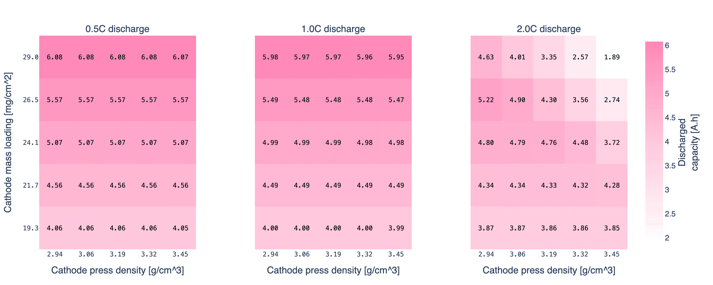
To show what this buys you in practice, we swept the cathode mass loading and press density across a 5×5 grid, with the anode loading scaled in step so the N/P ratio stays constant. At each grid point we measured the cell's actual capacity at C/10 (because the nominal 5 Ah from Chen2020 no longer applies once you change the electrode dimensions), then discharged at 0.5C, 1C, and 2C relative to that measured capacity.
The grid covers 19 to 29 mg/cm² on the cathode (0.8x to 1.2x the Chen2020 base) and 2.94 to 3.45 g/cm³ on press density (0.92x to 1.08x base, which runs from porosity ≈ 0.39 down to ≈ 0.28). These are ranges a cell designer might realistically consider when tuning a nickel-rich cathode for a new format. The simulations use PyBaMM's DFN with the Chen2020 parameter set, everything else held fixed.

At 0.5C the picture is simple. Capacity is controlled by loading (more grams of active material, more Ah) and press density barely matters, because the discharge is slow enough that electrolyte transport is not a bottleneck. The entire grid sits within 2% of the C/10 calibration capacity.
At 1C the story is still mostly sizing. Every point in the grid delivers between 96% and 97% of its C/10 capacity. Physics-based modelling at 1C, for this design window, would tell a cell designer that press density is a free variable, and inside this range it roughly is. A modelling team running only a 1C rate check would conclude that press density does not matter. That conclusion is true until it is not.
At 2C the grid starts to tilt. The Chen2020 base point (24.1 mg/cm², 3.19 g/cm³) holds 93% of its C/10 capacity. Keep the base mass loading but push press density to 3.45 g/cm³ and retention drops to 72%. Push mass loading to 29 mg/cm² as well and retention falls to 31%. The effect is gradient, not a cliff: moving one step in either direction costs 5 to 15 percentage points of retention, and the moves compound.
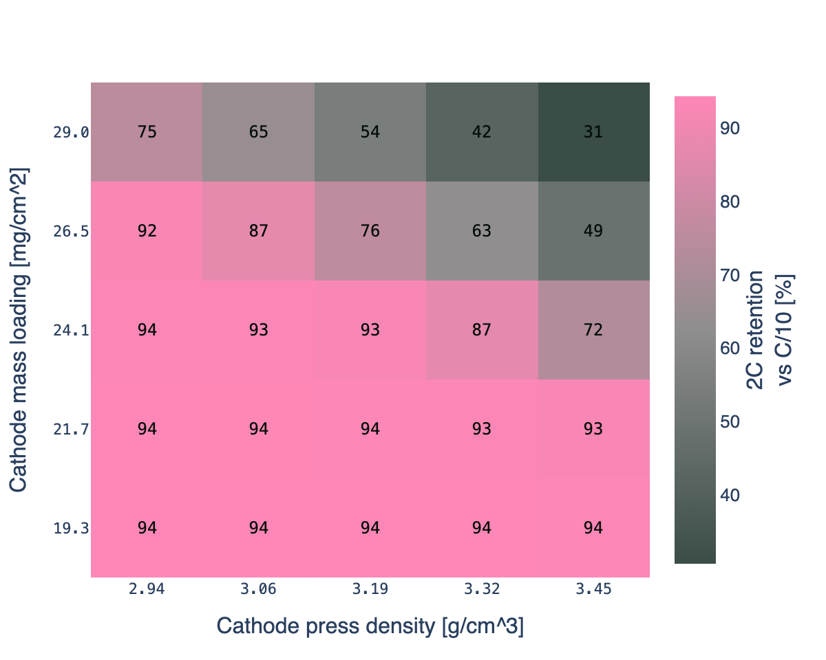
Three regions on the 2C map:
- Holds rate. Low mass loading or low press density. The electrolyte has enough pore volume to transport ions at 2C. Retention above 90%. Most of the grid.
- Borderline. Moderate loading at the higher press densities, or high loading at moderate press densities. Retention between 60% and 90%. Small moves in either input move you through this region.
- Transport-limited. High loading combined with high press density. Retention between 30% and 50%. The cell still has all the active material, but at 2C it cannot move enough lithium through the shrinking pore network to sustain the current before the voltage cutoff.
Press density matters here in a way it did not at 0.5C or 1C. The top row of the heatmap (29 mg/cm²) goes from 75% retention at 2.94 g/cm³ down to 31% at 3.45 g/cm³: a physically identical active-material inventory, 2.4x difference in accessible capacity at 2C, because the electrolyte pathway shrank. That is the kind of design lever a physics-based model lets you quantify before you build the electrode.
What the discharge curves look like
Four representative design points make the effect concrete. We pick:
- A. Thin (ML ×0.8, PD ×1.0): 19.3 mg/cm² at base density, smaller but with extra transport headroom
- B. Base (ML ×1.0, PD ×1.0): Chen2020 as published, 24.1 mg/cm² at 3.19 g/cm³
- C. Thicker (ML ×1.2, PD ×1.0): 29 mg/cm² at base density, more energy with no compaction change
- D. Thicker and denser (ML ×1.2, PD ×1.08): 29 mg/cm² at 3.45 g/cm³, pushing energy density
and run the 0.5C, 1C, 2C rate test on each.
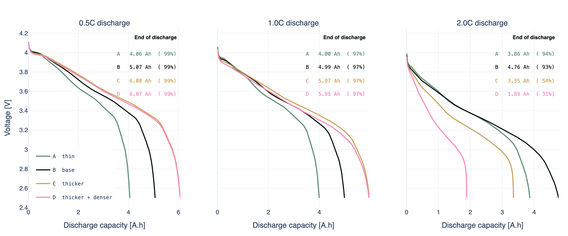
At 0.5C the four curves are essentially scaled copies of each other: same voltage profile, different total capacity. This is the regime most rate datasheets describe, and it is why a small rate test can mislead. Nothing about the 0.5C panel predicts the shape of the 2C panel.
At 1C, all four designs lose 3 to 4% of capacity to overpotential, and the ordering is still just by mass loading. A 1C test, by itself, would not tell you anything useful about the press density trade-off.
At 2C the separation becomes clear. A (thin, 19.3 mg/cm²) is virtually unchanged from its 0.5C curve because there is always enough electrolyte-phase transport headroom. B (base) holds most of its capacity with a slightly steeper sag. C (thicker, 29 mg/cm², base density) stops around 3.4 Ah, noticeably short of its 6.1 Ah 0.5C capacity, but still usable. D (thicker, 3.45 g/cm³) collapses to below 2 Ah even though it contains the same active material as C, because at higher press density the pore network can no longer sustain the ionic flux the current demands.
If you were optimising for pack energy density you would naturally pull in the direction of D. At 0.5C, D and C deliver the same capacity, but D does it in a smaller volume. At 2C, D gives you roughly half of what C does under load. That trade-off is impossible to see in datasheet-style nominal capacity, and it is the trade-off a physics-based model exists to quantify, provided the model is posed in the variables the designer actually adjusts.
Why this matters beyond one sweep
Physics-based battery models have been in research groups for decades, and for most mainstream chemistries the underlying physics is well understood. Adoption inside cell manufacturers and pack builders is still patchy, and the reason is usually not the physics. It is the handoff. The people who produce the models, the people who parameterise them, and the people who make design decisions from them often live in different tools, different vocabularies, and different confidence levels about what the model is actually saying.
Every time a parameter set moves between those groups, something gets lost. A process engineer asks "what happens if I increase mass loading by 10%" and the modeller updates the thickness, possibly forgetting to rebalance the anode, possibly keeping porosity fixed even though the factory route to higher loading is to press harder, which lowers porosity. Six weeks later someone notices the simulation does not match the build, and nobody is sure whose step introduced the divergence. This is how physics-based models acquire the reputation of being "academic."
Linked parameters are a small, concrete fix for one slice of this problem. The model is stored with the same inputs a manufacturer adjusts, so the translation step goes away. A sweep over mass loading and press density is literally a sweep over those inputs, not a cascade of thickness-porosity-volume-fraction edits that need to be kept consistent by hand.
It is not the whole answer. Parameter fidelity, OCV quality, degradation fits, temperature dependence, and cycling validation all sit on top of this. But getting the inputs right is load-bearing. Every layer above it assumes you did.
BPX and the shared-model layer
Linked parameters sit at the inputs layer: one team, one chemistry, one parameter set, recast in the variables that team uses. The other half of the industry adoption problem is at the model layer: different groups using different models, formats, and conventions to describe nominally the same cell. Moving parameters between groups is hard even when everyone agrees on the physics, because the files they save and the conventions they use differ.
BPX is an open standard for physics-based battery model exchange. It defines a common, versioned format for parameterised cell models that engineering tools can read, write, and validate against. Ionworks is one of the groups involved in its development, alongside a growing list of OEMs, simulation vendors, and academic groups, and PyBaMM reads and writes BPX natively.
BPX addresses the question "how do two organisations share the same model." Linked parameters address the question "how does one organisation expose that model in the variables its own teams already use." The two are complementary. Industry-strength physics-based modelling needs both: a shared format so the model is portable, and a flexible input layer so each team can drive it without relearning someone else's vocabulary.
Running the sweep in this post required no code changes to PyBaMM, no special solver, and no rewriting of the parameter file. Four numeric inputs and three symbolic expressions per electrode, and the rate capability study became a sweep over the variables a manufacturer actually controls. Ionworks Studio makes that setup a few clicks rather than a Python session: you define the inputs, bind the derived quantities as expressions, and the link is stored inside the model file so every downstream user inherits it. Book a demo to see how teams use Studio to build parameter files that read in whichever vocabulary the next engineer on the chain needs to think in.
Continue reading