Degradation fits have a reputation for grinding for days. Each candidate parameter set requires simulating thousands of aging cycles, and a global optimizer needs thousands of those evaluations. The arithmetic is unforgiving. When a single forward run takes hours, the full fit takes weeks, and the work becomes manual trial and error rather than optimization.
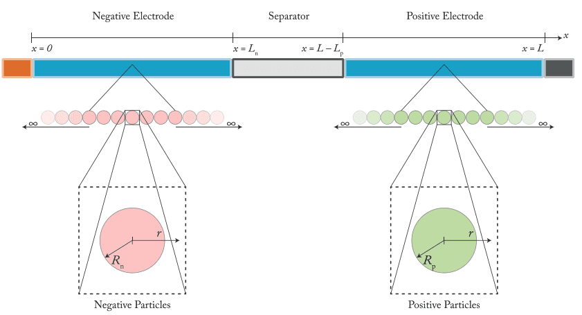
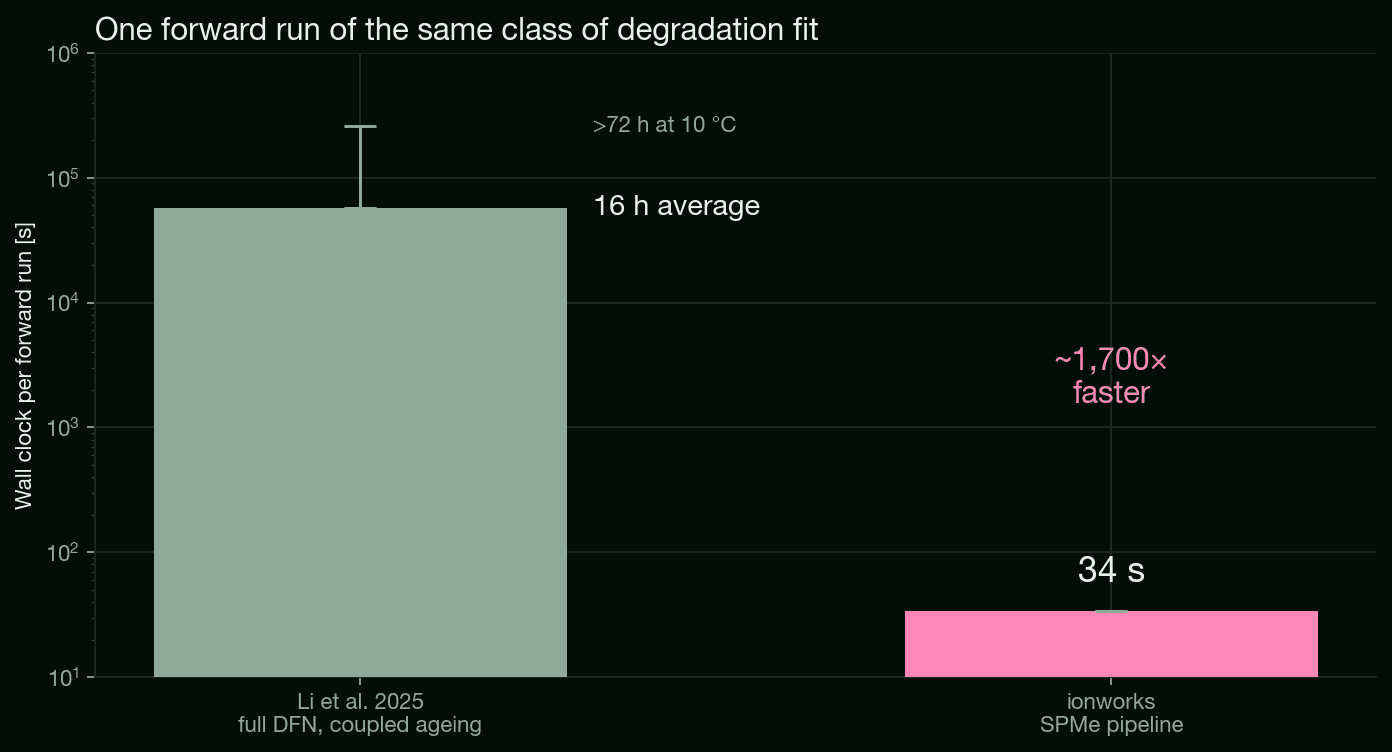
The Li et al. (2025) Nature Communications study on the LG M50 is a concrete reference point. They run a full DFN model with coupled physical degradation sub-models, SEI growth, lithium plating, cracking, and an electrolyte dry-out model, simulated cycle by cycle, where the end state of one cycle sets up the next. The authors report about 16 hours for one forward run of the fully coupled model, rising past 72 hours at 10 °C for some parameter combinations. The same class of fit on the Ionworks pipeline does one forward run in about 34 seconds, and the full global optimization converges in roughly six to seven hours on more than 100 cores.

That gap is large enough to invite the assumption that it is all model order. It is not. The biggest single factor was memory.
The unbounded memory growth that stalled everything
Early long runs grew memory without bound. A degradation fit simulates hundreds of cycles across several cells across many optimizer iterations, and a naive solver configuration stores the full internal state at every checkpoint. On a four-hour rest step that is hundreds of stored samples, multiplied by hundreds of cycles, multiplied by every cell. Resident memory climbed into the tens of gigabytes, the process began swapping to disk, and a run that should have taken hours ground to a halt against it.
The fix is almost never the integrator. It is knowing which quantities the fit actually needs and storing only those, at the points where they are read. Get that right and the solver keeps a handful of values per cycle and discards the rest, with no change to the physics being solved. It sounds obvious in hindsight. In practice it takes understanding both the metric definitions and the solver internals well enough to know exactly what is safe to drop, which is easy to get wrong and expensive to discover the hard way.
Profiled on a single evaluation of the joint fit, peak process memory fell from about 28 GB to about 0.35 GB.
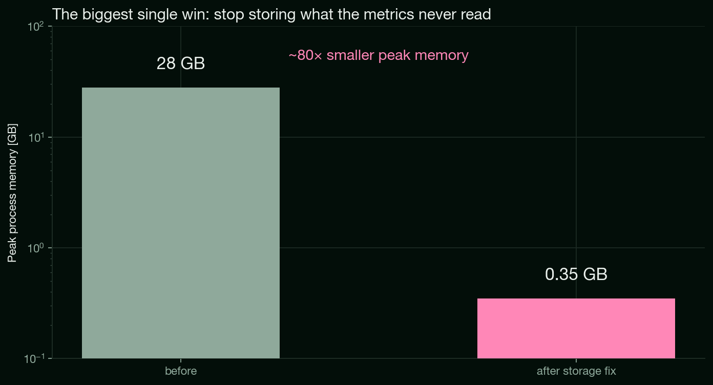
The number that matters here is peak memory, not total allocation. The high-water mark is what decides whether a fit runs or dies with an out-of-memory error. It dropped by roughly 80 times. Just as important, none of these changes is an approximation. They change what gets stored, not what gets computed. The final fit cost agreed to the last decimal place before and after. Flat memory bought two things at once: the runs stopped stalling, and there was now headroom to fit more observations per run instead of fewer.
The rest of the speedup
With memory under control, the other factors compound cleanly.

Model order does its share. SPMe instead of full DFN reduces the degrees of freedom by roughly a factor of ten, while keeping the degradation physics that the fit depends on. A single SPMe forward run is cheap, which is the precondition for running a global optimizer over it at all.
The optimizer is differential evolution, which evaluates an entire population of candidates that do not depend on each other. That independence is what makes it parallelize well. The platform distributes the work greedily across whatever cores are available, so a single optimizer evaluation runs 9,000 cycles, 3,000 at each of three temperatures, at the same time rather than in sequence.
None of these is exotic on its own. The combination is what turns a multi-week manual exercise into an overnight job, and the order matters: without the memory fix, parallelism just multiplies the swapping and the run never finishes.
That combination is the real point. Making a physics-based degradation fit this fast is less about any one trick than about knowing where the bottlenecks actually are, having built the model stack deeply enough to fix them at the source, and packaging the result so a team gets it by default instead of rediscovering it on every project. That is the work behind the Ionworks platform, done by the people who build and maintain PyBaMM. For more on how the fitting is set up, see our parameter estimation guide and our overview of computational approaches in battery R&D.
Frequently asked questions
Continue reading