Every battery modeling decision is a bet. You are betting that the physics you include will be sufficient to answer your question, and that the parameterization cost and compute time will be worth the answer you get. Too little physics and the answer is wrong. Too much and you spend weeks on parameterization for a question that a simpler model could have handled by Tuesday.
Battery R&D teams often land at one of two extremes. They rely on ECMs and Excel because those are fast and familiar, but too simplistic to base design decisions on. Or they assume physics-based models require a PhD in electrochemical modeling and custom scripts that only one engineer understands. Neither extreme is necessary. The real question is which level of physics your engineering question actually requires.
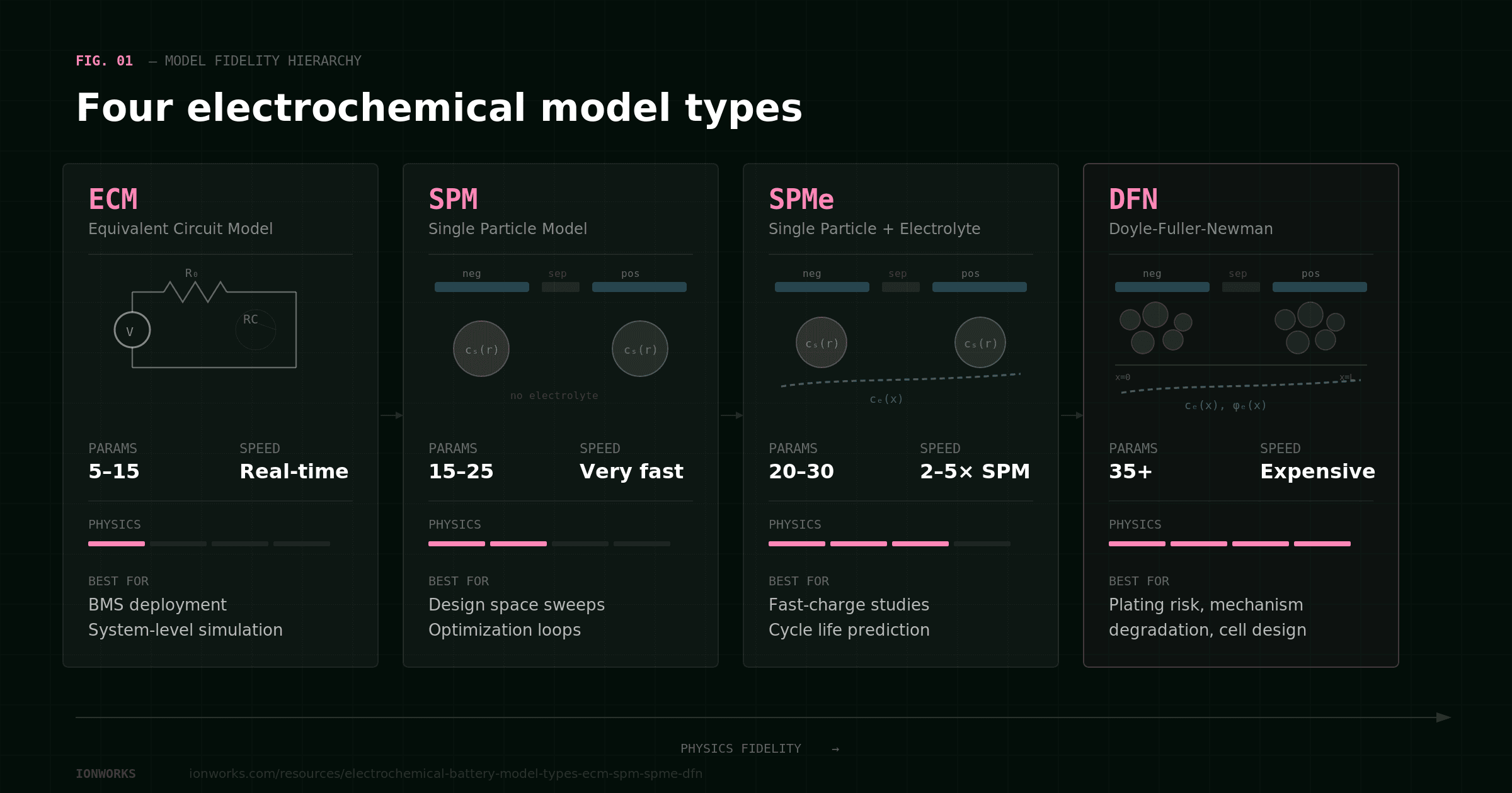
The four electrochemical model types in PyBaMM form a clear hierarchy: ECM, SPM, SPMe, and DFN, in order of increasing physics, increasing parameterization burden, and increasing computational cost. The right choice depends on what you are trying to predict. Not all of these models are equally good at all tasks, and pretending otherwise wastes engineering time.
The model hierarchy at a glance
The progression is straightforward. ECM treats the cell as a black-box circuit element. pybamm.lithium_ion.SPM() introduces solid-phase diffusion physics but ignores the electrolyte. pybamm.lithium_ion.SPMe() adds electrolyte concentration gradients and ohmic losses through the separator. pybamm.lithium_ion.DFN() resolves spatial transport across the full electrode thickness, giving access to gradients that the reduced-order models average away.
Each step up buys you more internal variables and better accuracy at high rates, but costs more data and more compute. The rest of this guide walks through each model so you can match model fidelity to your actual engineering question.
ECM (Equivalent Circuit Model)
What it captures
The canonical ECM is a first-order Thevenin circuit: a SoC-dependent OCV source in series with an ohmic resistance and one or more RC pairs. It is purely empirical. There are no electrodes, no particles, no electrolyte. The model reproduces terminal voltage as a function of current and SoC, and that is all it does.
Parameterization
ECM parameterization is fast. You need time-series voltage and current data, typically from HPPC pulse tests and a slow OCV curve. The total parameter count lands somewhere between 5 and 15, depending on how many RC pairs you use. No teardown, no half-cell experiments, no electrolyte characterization. If you have cycling data, you can have a parameterized ECM the same day.
Computational cost
ECMs run in real time on embedded hardware. This is their reason for existing in deployed BMS systems. Ionworks exports ECMs directly to Simulink, MATLAB, and C++, making the path from parameterization to deployment straightforward.
When to use ECM
ECM is the right model for real-time SoC and SoH estimation on embedded controllers, for system-level simulation where cell fidelity is secondary to pack or vehicle behavior, and for early-stage project scoping when cycling data is all you have.
Where ECM falls short
An ECM cannot tell you what is happening inside the cell. Anode potential, lithium plating risk, SEI growth rate, electrolyte depletion: none of these are accessible. It cannot distinguish between electrode-specific behaviors, and it does not separate the contributions of the anode and cathode to the overall voltage response.
ECM predictive accuracy is also limited to interpolation within the training data. If you fit an ECM to 25°C cycling at 1C and then simulate 0°C at 3C, the extrapolation has no physics to lean on. An ECM can fit a capacity fade curve, but it cannot explain why the cell is degrading or what design change would fix it. If your question requires any internal variable, ECM is the wrong tool.
SPM (Single Particle Model)
What it captures
SPM represents each electrode as a single spherical particle. It models solid-phase lithium diffusion within those particles and intercalation kinetics at the electrode-electrolyte interface. Current distribution across the electrode thickness is assumed uniform, and electrolyte dynamics are ignored entirely. This is the simplest physics-based electrochemical model available.
A key advantage over ECM: SPM tracks separate OCV curves and transport parameters for the anode and cathode. This means you can inspect electrode-specific overpotentials (diffusion, kinetic) and identify which electrode limits performance under a given protocol. That diagnostic capability is entirely absent in an ECM.
Parameterization
You need a full-cell OCV curve (to extract electrode OCV curves and capacities), rate capability data at several C-rates, and HPPC or GITT pulse data for diffusion and kinetic parameters. No teardown and no half-cell experiments are required. The parameter count is moderate (roughly 15 to 25). Our parameter estimation guide covers the full SPM data requirements and explains how lumped parameterization fits the dimensionless groups that full-cell data can actually resolve, rather than trying to recover individual physical quantities the experiment cannot constrain.
Computational cost
SPM solves a single PDE for solid diffusion, with algebraic equations for everything else. It is the fastest physics-based model in PyBaMM and well suited for large parameter sweeps and optimization loops where you need thousands of simulations to converge on a design.
When to use SPM
SPM works well for design space exploration at moderate C-rates: sweeping electrode thickness, particle radius, or capacity loading to identify promising regions before committing to higher-fidelity studies. Its speed makes it natural for optimization loops.
Where SPM falls short
SPM accuracy degrades above roughly 1C for most chemistries. Without electrolyte dynamics, the model cannot capture concentration-dependent overpotentials that dominate at high rates. JuliaSimBatteries benchmarks show SPM producing visible differences in voltage, current, average temperature, and SoC relative to DFN during fast-charge simulations. Degradation fidelity is also limited: SPM lacks the electrolyte transport physics needed for realistic SEI growth or plating models.
SPMe (Single Particle Model with Electrolyte)
What it captures
SPMe extends SPM by adding electrolyte concentration gradients and the potential drop across the separator. It still uses a single-particle representation per electrode, so there is no spatial distribution within the electrode. But the electrolyte coupling captures transport limitations that SPM misses, and the accuracy improvement at moderate-to-high C-rates is significant.
Parameterization
SPMe requires everything SPM needs, plus electrolyte transport parameters: diffusivity and ionic conductivity. For common electrolyte systems these can often be sourced from literature. No teardown or half-cell data is required. The data burden is incrementally higher than SPM, not qualitatively different. (The parameter estimation guide covers the SPMe-specific additions.)
Computational cost
SPMe adds PDEs for electrolyte transport, making it roughly 2 to 5 times slower than SPM. It remains much faster than DFN. The same JuliaSimBatteries benchmarks that show SPM diverging from DFN at fast-charge rates report SPMe "in great agreement with the DFN model" for NMC cells. That accuracy-to-cost ratio makes SPMe the workhorse for many practical studies.
When to use SPMe
SPMe is the right starting point for fast-charge envelope studies where you need to evaluate protocols across temperature and rate but do not yet need spatially resolved plating risk. It is also well suited for calendar aging studies, cycle life prediction, and any work where intermediate fidelity will answer the question.
SPMe and degradation
SPMe handles degradation modeling well. The electrolyte dynamics it includes enable realistic SEI growth and capacity fade models that SPM cannot support. Mode-level degradation analysis (LLI, LAM, resistance growth) runs well on SPMe, and for many calendar aging and cycle life studies, SPMe provides sufficient fidelity without the parameterization cost of DFN.
Where SPMe falls short is mechanism-level degradation that depends on spatial gradients within the electrode. Lithium plating risk varies with position: it peaks near the separator where lithium flux is highest. DFN resolves that gradient. SPMe does not.
DFN (Doyle-Fuller-Newman Model)
What it captures
The DFN model implements full porous electrode theory. Both electrodes are treated as porous media with spatially resolved transport in the electrolyte and solid phases. Intercalation kinetics, charge conservation, and species transport are all coupled across a 1D domain spanning the anode, separator, and cathode. Every degradation submodel available in PyBaMM (SEI, lithium plating, LAM, particle cracking) attaches to the DFN framework.
Spatial resolution: the key differentiator
The defining advantage of DFN over the reduced-order models is spatial resolution within the electrode. Anode potential is not uniform across the electrode thickness. Near the separator, where lithium flux peaks during charging, the anode potential drops lower than near the current collector. Plating risk is highest in that region, and DFN captures the gradient that determines whether plating occurs and where. SPM and SPMe average over the electrode thickness and cannot see this.
The same principle applies to non-uniform porosity in graded electrode architectures, to reaction rate distributions that shift with C-rate and temperature, and to electrolyte depletion profiles that vary spatially through the electrode and separator. If your question involves where something happens within the electrode, not just whether it happens, DFN is required.
Parameterization
DFN parameterization is the heaviest in the hierarchy. It requires half-cell OCV curves, a full-cell OCV characterization, cell teardown for geometric parameters (electrode dimensions, particle sizes, porosities, active material volume fractions), and rate capability tests to fit transport and kinetic properties as functions of temperature and SoC. Chen et al. 2020 demonstrated 35+ parameters for a single LG M50 21700 cell. A solver can run in seconds. Assembling a defensible parameter set often takes weeks.
Our battery parameter estimation guide walks through the full step-by-step data requirements for DFN, SPM/SPMe, and ECM parameterization, including what makes each step necessary and where identifiability problems hide.
Ionworks treats parameterization as a first-class workflow: global optimization with multistart, uncertainty quantification, Bayesian priors, and full provenance of where each parameter came from and how it was estimated. That infrastructure matters most at DFN scale, where the parameter count is high enough that manual bookkeeping breaks down.
Computational cost
DFN is the most expensive physics-based model in PyBaMM. It solves coupled PDEs for solid diffusion in both electrodes plus electrolyte transport. Individual simulations are tractable. Large parameter sweeps or optimization loops are expensive, and this cost shapes how teams use DFN in practice: targeted studies where the spatial physics matter, not broad screening.
When to use DFN
DFN is the right model when lithium plating risk must be quantified (you need the anode potential spatial profile, not just a cell-averaged value), when mechanism-level degradation studies require spatially resolved SEI or cracking, when you are optimizing electrode thickness, porosity, or loading, and when graded electrode architectures are under consideration. DFN also serves as the reference model for validating reduced-order models like SPM and SPMe.
Beyond 1D DFN
Standard DFN assumes a single active material per electrode and a monotonic OCV curve. Several important chemistries and cell geometries violate those assumptions.
Composite electrodes
Graphite-silicon blends are the most common case. PyBaMM's BasicDFNComposite models each active material phase with its own particle diffusion and OCV curve, capturing the differential lithiation between graphite and silicon domains. Without a composite model, the silicon contribution to capacity and degradation is averaged away.
Hysteresis models
LFP and silicon chemistries exhibit significant OCV hysteresis: the voltage on charge differs from the voltage on discharge at the same SoC. Standard models assume a single OCV curve. PyBaMM includes hysteresis state models that track the charge/discharge branch. These matter for SoC estimation accuracy and for degradation prediction in LFP cells where path-dependent voltage errors accumulate.
MSMR (Multi-Species Multi-Reaction)
The MSMR framework (Yang et al. 2017) models multiple intercalation reactions within a single electrode particle. This captures graphite staging plateaus and NMC phase transitions with higher thermodynamic accuracy than a fitted polynomial OCV. The tradeoff is a higher parameterization burden: each reaction species requires its own thermodynamic and kinetic parameters.
3D electrochemical models
Large-format pouch and prismatic cells have in-plane gradients that 1D models cannot see. Tab placement affects internal resistance distribution. Temperature hotspots localize near tabs or at cell centers. Structured electrodes introduce geometric complexity. Pseudo-3D and full 3D electrochemical models resolve these gradients. Ionworks offers full 3D simulation where the same parameterized model extends from 1D to 3D without rewriting, avoiding the common workflow of maintaining disconnected parameter sets across tools.
Model selection by use case
Fast charge
SPMe handles fast-charge protocol development when you need to evaluate rate and temperature envelopes. The electrolyte physics it captures are sufficient for identifying protocols that avoid obvious thermal or voltage limits. When lithium plating risk is the primary concern, DFN is required. Plating prediction needs the anode potential spatial profile near the separator, and SPMe does not resolve that. For teams running protocol sweeps, Ionworks Predict supports both model types with the same simulation interface.
Degradation modeling
ECM can fit capacity fade curves to cycling data, but the fitted parameters have no mechanistic meaning. You cannot use an ECM to distinguish between LLI, LAM, and resistance growth, let alone design a fix. SPMe supports mode-level degradation analysis and is a reasonable choice for calendar aging, cycle life screening, and resistance growth studies. DFN is required for mechanism-level degradation: SEI spatial distribution, plating onset conditions, particle cracking, and coupled multi-mechanism studies like those demonstrated by O'Kane et al. 2022.
Electrode and cell design
SPM is fast enough for first-pass design sweeps over electrode thickness, particle size, and capacity loading. When you need to optimize porosity profiles, graded architectures, or formation protocols, DFN gives you sensitivity to the microstructure parameters that SPM averages away. The battery simulation software comparison covers how different tools handle these workflows.
BMS deployment
ECM remains the standard for real-time embedded SoC and SoH estimation. SPM and SPMe are increasingly used in advanced physics-aware BMS architectures where internal state estimates (solid-phase concentration, for example) improve control decisions. DFN is too expensive for real-time embedded use in most implementations, but it serves as the reference model for validating reduced-order BMS algorithms offline. See our BMS simulation resource for a deeper treatment.
Tradeoff matrix
| Dimension | ECM | SPM | SPMe | DFN |
|---|---|---|---|---|
| Physics captured | Terminal voltage only | Solid diffusion, kinetics | + Electrolyte transport | Full porous electrode theory |
| Parameterization burden | Low (5-15 params, no teardown) | Moderate (full-cell data only) | Moderate+ (add electrolyte params) | High (teardown + half-cell, 35+ params) |
| Compute cost | Real-time on embedded HW | Very low (1 PDE) | Low-moderate (2-5x SPM) | High (all PDEs, expensive for sweeps) |
| Degradation capability | Fits fade curves, no mechanism | Limited (no electrolyte physics) | Good (mode-level: LLI, LAM, resistance) | Full (mechanism-level: SEI, plating, cracking) |
| Design optimization | None | First-pass sweeps | Intermediate fidelity | Full electrode microstructure |
| BMS suitability | Standard for embedded | Advanced physics-aware BMS | Advanced physics-aware BMS | Reference/validation only |
From PyBaMM scripts to a production workflow
Most teams working with PyBaMM follow a familiar arc. You start with a Jupyter notebook running pybamm.lithium_ion.SPM(), move to SPMe or DFN as the questions get harder, and eventually need to export a reduced model for BMS deployment or run 3D simulations for a large-format cell design.
At each transition, the parameter set changes tools. The SPM parameters live in a Python dict. The 3D model lives in a general-purpose multiphysics tool with its own parameter format. The BMS ECM lives in a system-level simulation environment. Nothing connects them, and reproducibility depends on whoever last touched the spreadsheet.
Ionworks was built to close that gap. It supports ECM through DFN, degradation submodels, and 3D electrochemical simulation in a single platform, built directly on PyBaMM by the team that created PyBaMM. There is no translation layer between the open-source solver and the production workflow.
Parameterization in Ionworks records the model type, the validated parameter set, and the cell specification together, with full provenance of where each parameter came from and how it was estimated. Teams can reuse and trust each other's results because the parameter sets are versioned and traceable.
When a model needs to move downstream, Ionworks exports to Simulink, MATLAB, and C++ for BMS integration. When a 1D DFN study needs to extend to 3D for a large-format cell, the same parameterized model carries over without rewriting. The alternative is maintaining three disconnected parameter sets across PyBaMM scripts, a multiphysics tool for 3D, and a system-level environment for BMS, and hoping they stay consistent.
As battery engineering teams move from research prototyping to production modeling, the bottleneck is rarely solver speed. It is parameterization discipline, model reproducibility, and workflow continuity across fidelity levels. That is the layer Ionworks adds around PyBaMM.
Frequently asked questions
Continue reading