Why we fit degradation modes, not capacity

A team fits a physics-based model to a capacity-fade curve. The fit looks good. Every point sits close to the line. Then they extrapolate a few thousand cycles past the training window, or move to a cell aged at a different temperature, and the prediction drifts. The parameters that fit one cell do not transfer to the next. Refit, and a different combination of parameters lands on the same curve.

This is the trap of fitting capacity directly. Capacity is one number, and it is the net result of several aging mechanisms moving at the same time. When you score a fit against capacity alone, the optimizer is free to reach the right total through the wrong combination of mechanisms. The cost function cannot tell the difference. You get a model that reproduces the training data and predicts badly the moment conditions change.

The fix is to stop treating capacity as the fitting target and start treating it as a consequence.

Capacity is a projection

A lithium-ion cell loses usable capacity through a handful of distinct mechanisms. Lithium gets locked into the SEI and into dead lithium from plating, which is loss of lithium inventory (LLI). Active material is lost at each electrode through particle cracking and isolation, which is loss of active material at the negative and positive electrodes (LAM_neg and LAM_pos). Internal resistance rises as interfaces grow and contact degrades.

Each of these has its own rate, its own temperature dependence, and its own response to the cycling protocol. The capacity you measure at a reference test is the projection of all of them onto a single axis. Two cells can show the same capacity fade while one is plating-limited and the other is losing cathode active material. Their futures are completely different. Their capacity curves, today, are identical.

The figure below shows a single cell at 25 °C. The top panel shows a single result: one capacity-fade curve. The bottom panel is what is actually happening underneath it, the four modes recovered separately by differential model analysis.

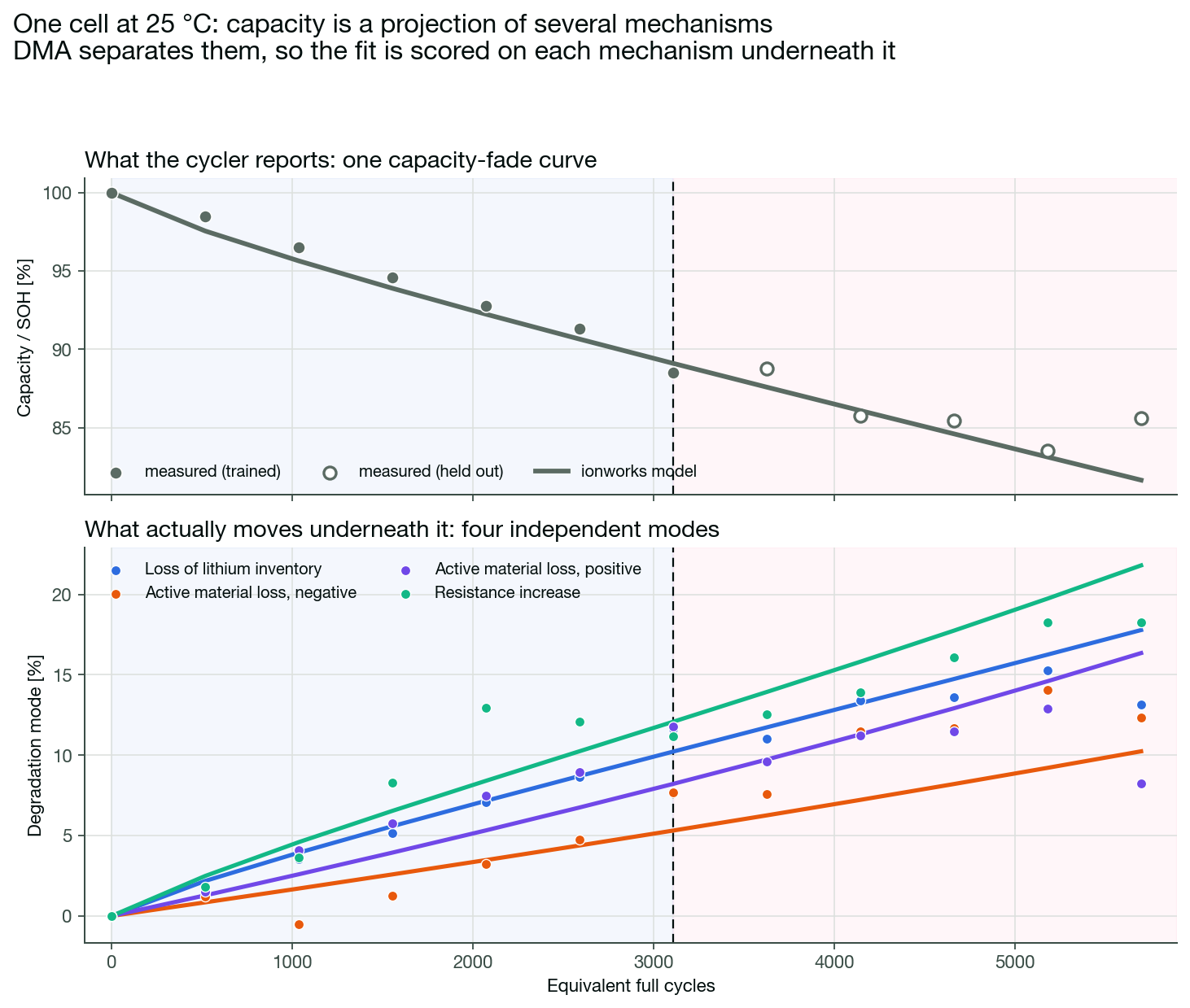
Differential model analysis (DMA), for example in Dubarry et al. (2012), is the standard way to recover those modes from slow-rate voltage curves. It fits the full-cell open-circuit voltage as a combination of the two electrode curves, then tracks how the electrode capacities and their relative alignment shift over life. Loss of alignment is LLI. Shrinking electrode capacities are LAM. The resistance metrics come from the pulse response. The mechanisms come out of the same reference performance tests teams already run.

Modes as the fitting target

Once the modes are separated, they become the fitting target. Each cell contributes four mode trajectories plus capacity, and the model is scored against all of them. The optimizer can no longer trade a too-fast plating rate against a too-slow cathode loss to land on the right capacity, because both errors are now visible and penalized independently. The fit is far more constrained, which is exactly what you want when several parameters are otherwise collinear.

This is the case Li et al. (2025) make directly. Their paper is about the importance of degradation mode analysis in parameterizing lifetime models, and the reason is physical. The parameters you recover by fitting the modes map onto real mechanisms: the SEI growth rate, the plating kinetics, the active-material loss rate at each electrode. A converged fit is then more than a curve that matches. It is an explanation. It tells you which mechanism dominates, at which temperature, and at what point in life one overtakes another. A capacity-only fit can reproduce the same curve and stay silent on every one of those questions.

That physical grounding is the whole point. The output is not a black-box parameter set tuned to one cell, it is a set of mechanism rates you can read, compare across conditions, and carry to a cell or duty cycle you have not tested yet.

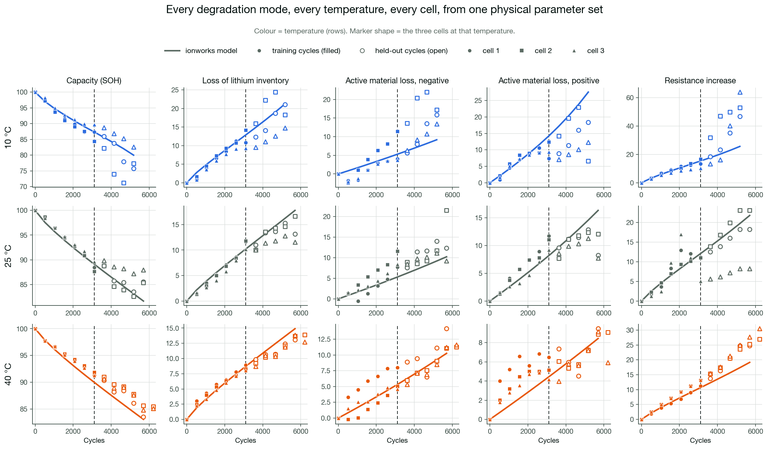
For the public LG M50 dataset from Li et al., we fit a single SPMe model with SEI growth, lithium plating, and stress-driven active material loss. Every one of these mechanisms is available in public PyBaMM. The source paper extends PyBaMM with an additional electrolyte dry-out model; here the public mechanisms were sufficient. Seven physical parameters are fitted jointly across three ambient temperatures (10, 25, and 40 °C), and we hold out entire cells and the back half of every cell's cycle history, so the validation is genuinely out of sample.

One parameter set has to reproduce every mode, at every temperature, for every cell.

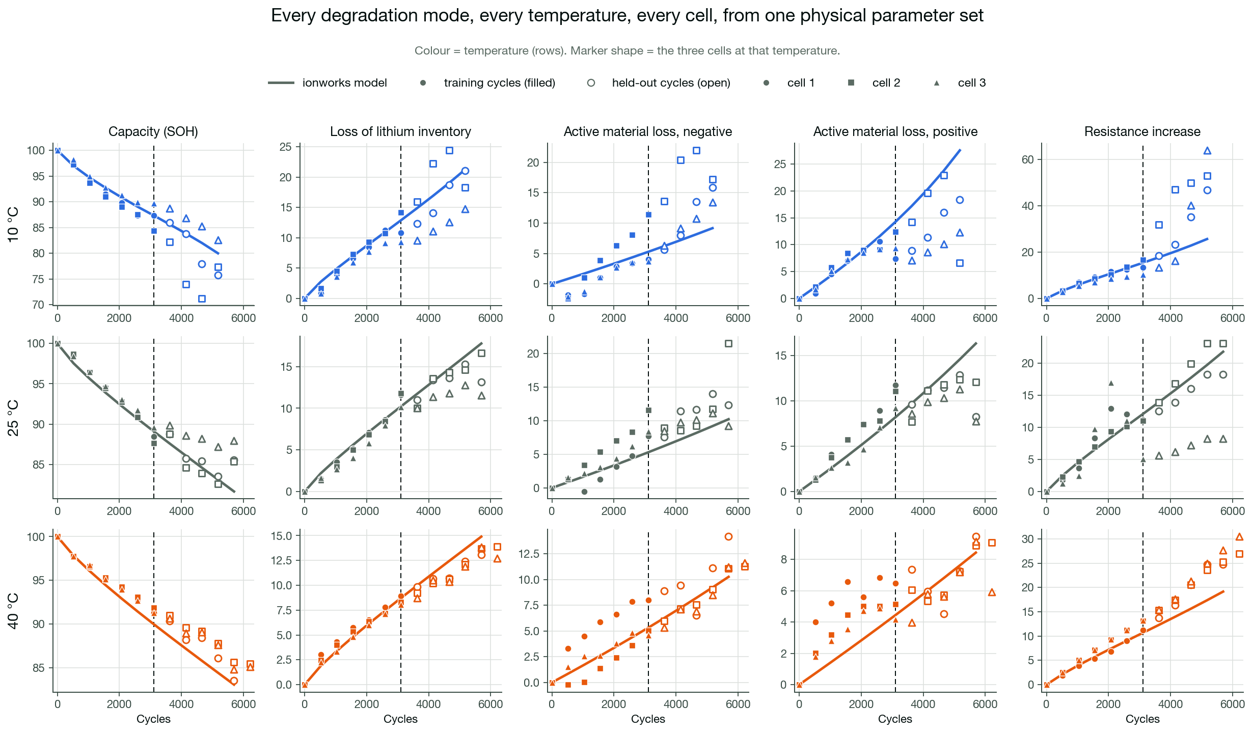
How it holds up

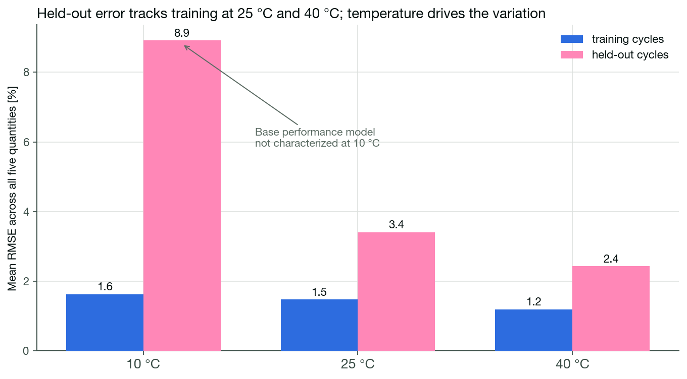
The fit generalizes. Trained on cycles up to roughly 3,100, it predicts held-out cells out to about 6,200 cycles, and the held-out error stays close to the training error. Temperature is the main axis of variation, and the train-versus-test gap stays small by comparison. The 25 °C and 40 °C cells are reproduced tightly, and the larger error at 10 °C reflects the base electrochemical model, whose performance parameters were not characterized at 10 °C. That uncertainty lives in the base model, separable from the degradation fit and addressed by characterizing the base model at 10 °C.

Fitting the modes is what makes this readable. Because each mechanism is fit independently, you can see where the model is strong, where it is uncertain, and which physical input to improve next. The mechanisms behind these modes, and how to set up the reference tests that expose them, are covered in our degradation and parameter estimation guides. If you are running lifetime fits and want parameters you can actually reason about, the fitting target is the first thing to change.