Battery aging and degradation simulation: a guide for battery engineers
Battery lifetime prediction is hard. Not because the physics is unknown — the mechanisms are well-characterized in the literature — but because the interactions between them are complex, the relevant parameters are difficult to measure, and the timescales involved make experimental validation expensive.
A cell that will last 1,000 cycles takes roughly two years to test at one cycle per day. A cell that will last 2,000 cycles takes four. If the design changes partway through — a new electrolyte additive, a different formation protocol, a shift in electrode loading — the clock resets.
Simulation does not eliminate the need for testing. It changes what testing is for.
Three questions, three model classes
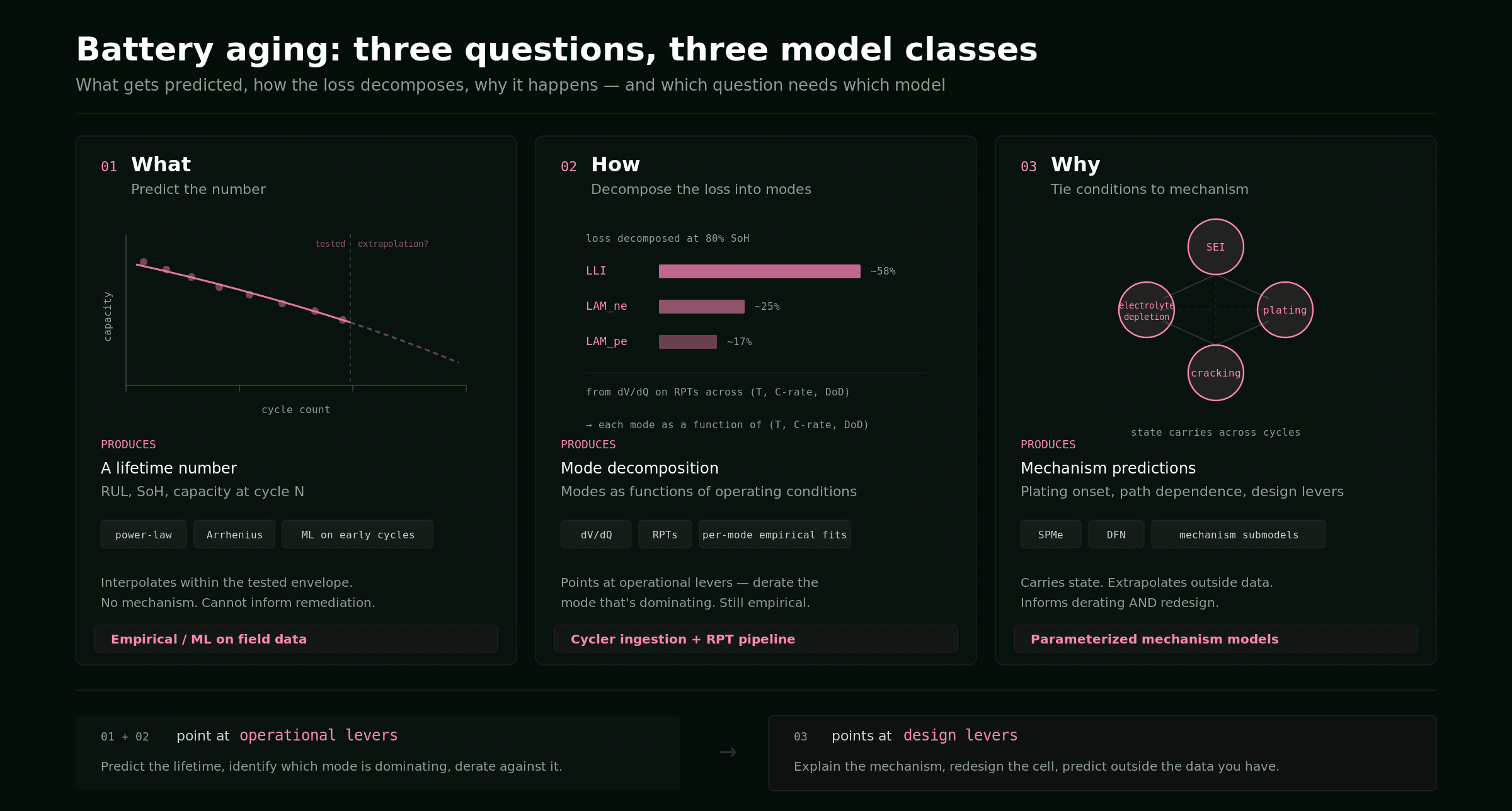
A lifetime question almost always reduces to one of three forms.
- What will happen — capacity at cycle 1,000, remaining useful life (RUL) at 80% SoH, warranty expectancy across a fleet? You want a number.
- How is the cell aging — how much of the loss is lithium inventory, how much is active material, how much is resistance growth? You want to decompose the loss.
- Why is it aging — what does each mechanism (SEI, plating, cracking, decomposition) do to the cell as operating conditions change? You want to tie conditions to physical processes, and predict outside the data you have.
Each question maps to a different class of model.
| Question | Approach | What goes in |
|---|---|---|
| What — predict lifetime within a tested envelope | Single empirical / ML model fit to capacity vs. cycle | Average T, DoD, C-rate, SoC window; sometimes early-cycle features |
| How — separate the loss into modes | Empirical models per mode | LLI(T, C-rate, DoD), LAM_ne(T, C-rate, DoD), LAM_pe(T, C-rate, DoD) — fitted from periodic dV/dQ on cycling data |
| Why — tie conditions to mechanisms | Physics-based electrochemical model with degradation submodels | SEI growth equation, plating reaction, particle-cracking model, electrolyte decomposition — each with its own rate law |
The dividing line between how and why is whether a degradation submodel is involved. Per-mode empirical fits give you LLI(T, C-rate) without ever simulating SEI growth. Mechanism submodels do simulate it — and that is what lets the model tell you what happens when the conditions move outside the data.
For most R&D questions, start with SPMe plus mechanism submodels (the why class). It is fast enough for long aging trajectories, captures cross-mechanism coupling through state variables, and parameterizes from full-cell data without teardown. DFN is the step up only when spatial gradients inside the electrode drive the answer.
Modes vs. mechanisms: keep the distinction sharp
A degradation mode is what is observable at the cell terminals. A degradation mechanism is what is happening inside the cell.
Three modes describe almost all observable aging:
| Mode | What it measures | Mechanisms that can cause it |
|---|---|---|
Loss of lithium inventory (LLI) | Lithium permanently removed from the active inventory | SEI growth, lithium plating (dead lithium), electrolyte depletion |
Loss of active material at the negative electrode (LAM_ne) | Anode material no longer available for intercalation | Particle cracking (graphite fracture, silicon expansion), contact loss |
Loss of active material at the positive electrode (LAM_pe) | Cathode material no longer available for intercalation | Particle cracking, structural change, transition-metal dissolution |
The four mechanisms that drive most observable aging in lithium-ion cells are SEI growth, lithium plating, particle cracking, and electrolyte depletion. Resistance rise is best understood as an emergent observable — not a primary mode but a consequence of SEI thickening, contact loss from cracking, and electrolyte depletion all raising the internal impedance.
The same mode can be produced by different mechanisms. LLI driven by SEI growth has square-root-of-time kinetics, mild temperature sensitivity, and weak rate dependence. LLI driven by plating has sharp temperature and rate thresholds and is path-dependent on prior cycling. A model that fits LLI from cycling data captures how much; it does not capture which. Two cells with identical LLI trajectories under one protocol can diverge under another, because the underlying mechanisms scale differently with conditions.
This is why the model class has to match the question. If you only need to extrapolate within the conditions you have tested, the mechanism does not matter — fit the curve. The moment a new protocol, chemistry, or operating window is on the table, the mechanism is the answer.
Predicting what: empirical and ML lifetime models
Empirical lifetime models — power-law or Arrhenius-based functions fit to capacity vs. cycle number — are fast, interpretable, and require minimal parameterization. They work well for warranty modeling and fleet-level SoH estimation when the operating conditions are consistent with the data they were fit on.
ML models trained on large cycling datasets capture interactions between temperature, C-rate, SoC window, and aging rate that are difficult to encode in closed-form equations. Severson et al. 2019 showed that ML models can predict RUL from the first 100 cycles within roughly 9% error — useful for cell screening and quality control on a known chemistry and form factor.
Use empirical and ML when:
- The operating envelope is stable and well within tested conditions.
- You need a number quickly across many cells (fleet SoH, warranty, screening).
- You do not need to know which mode or mechanism is driving the fade.
They break when:
- The duty cycle is path-dependent. Calendar storage then cycling, formation changes, mid-life protocol shifts — a capacity-vs-cycle fit carries no state, so it cannot represent a cell whose SEI thickness reflects six months of high-SoC storage before its first cycle, or one whose plated lithium from a cold fast-charge accelerates the rest of its life. Two cells with the same average T, DoD, and C-rate but different histories will share an empirical curve and diverge in reality.
- You need to act on the answer. A what model returns a number. It does not say which mode is dominating or which mechanism is driving the loss, so it cannot tell you whether to derate the upper voltage, slow the fast-charge ramp at low SoC, change the electrolyte additive, or rebalance the electrode loadings. Remediation — operational or by design — needs how or why.
Decomposing how: empirical models per mode
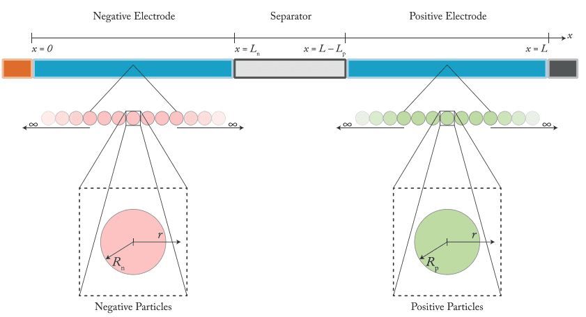
A step up from a single capacity-vs-cycle fit is to decompose capacity loss into modes — LLI, LAM_ne, LAM_pe — and fit empirical relations for each. The decomposition usually comes from periodic reference performance tests (RPTs): low-rate voltage curves taken every N cycles, processed with differential voltage analysis (dV/dQ) or incremental capacity analysis (dQ/dV) to separate full-cell capacity loss into anode-side and cathode-side contributions.
What you get from this is a set of empirical surfaces — LLI(T, C-rate, DoD, cycle count), LAM_ne(T, C-rate, DoD, cycle count), LAM_pe(...) — fitted across the cells in your test matrix. Resistance growth from EIS or HPPC can be added as a fourth empirical surface where it matters. Tools that focus on this decomposition (Ridgetop's CellSage is one example) operate primarily here.
Use per-mode empirical fits when:
- You have a test matrix that spans the operating conditions you care about, with periodic RPTs on every cell.
- You want to identify which mode is dominant so you can act on it. Mode dominance points to operational remediation: if
LAM_peis the bottleneck, derate the upper cutoff voltage; ifLLIfrom plating is the bottleneck, narrow the fast-charge SoC band or raise the lower temperature limit; ifLAM_nefrom silicon expansion is the bottleneck, ease the SoC swing. Per-mode fits give you the lever even without a physics parameterization. - You need a faster lifetime estimate for decisions where the conditions stay close to the data.
Where they stop:
- They cannot tell you whether the
LLIis going to SEI, dead lithium, or electrolyte depletion. The fit is to the mode, not to the cause. - They cannot extrapolate outside the conditions tested. A surface fit at 25–35°C does not predict 45°C, because the mechanisms that dominate change with temperature.
- They cannot capture path dependence. Calendar storage at high SoC followed by fast charging produces a different trajectory than fast charging from new — and a per-mode empirical fit on cycling data has nowhere to put the storage history.
Whenever any of those three limits is on the table — extrapolation, path dependence, or attribution to mechanism — the question becomes a why question.
Explaining why: mechanism submodels in a physics-based model
A why model attaches degradation submodels to a physics-based electrochemical model. Each submodel encodes a physical or chemical process: an SEI growth equation with diffusion-limited Arrhenius kinetics, a lithium plating reaction term tied to anode potential, a particle-cracking model coupled to lithiation strain, an electrolyte depletion term that consumes electrolyte through SEI formation and cathode-side oxidation. Each submodel has its own rate law, parameters, and dependencies on local state.
The defining property is that the model carries state through the simulation. SEI thickness, plated-lithium quantity, electrolyte concentration, fraction of cracked active material, electrode stoichiometry — all evolve over thousands of cycles, and each mechanism's rate at any moment depends on where the cell currently is, not just the average operating conditions. That is what ties operating conditions to degradation in a way an empirical fit on average T, DoD, and C-rate cannot.
The other thing mechanism submodels enable is design-level remediation. How models point at operational levers (derate the upper voltage, narrow the SoC window). Why models point at design levers: an electrolyte additive that suppresses SEI growth, an anode coating that reduces plating onset, a formation protocol that lays down a more stable SEI, a thicker separator or different porosity, a chemistry change. The mechanism is the design lever — and only a model that simulates the mechanism explicitly can tell you whether a candidate change will pay off across the conditions the cell will actually see.
Pure calendar aging is actually one of the places where empirical models hold up. Storage data across SoC × T combinations fits well to an Arrhenius surface with SoC-dependent prefactors, and that fit interpolates and extrapolates reasonably within the storage envelope. Storage-only lifetime is a what question.
Calendar aging becomes a why question the moment it composes with cycling — which it does in nearly every real duty cycle. A car is parked roughly 95% of the time and driven 5% of the time. A grid storage cell sits at high SoC for most of the day and dispatches intermittently. The SEI thickness when the cell enters a drive or dispatch phase reflects the prior storage; the rate of plating and SEI cracking during the active phase depends on that thickness; the SEI laid down during the active phase sets the starting point for the next storage interval. The combined trajectory is not the sum of a calendar curve and a cycling curve — there is no purely empirical way to compose them, because the rate in each phase depends on state that the other phase left behind. SEI thickness, plated-lithium quantity, and electrolyte concentration are state variables that mechanism submodels carry across phases. Empirical fits cannot.
The four mechanisms that matter most in lithium-ion cells:
- SEI growth has two components — calendar (thermodynamic, diffusion-limited, square-root-of-time, strong T and SoC dependence) and cycle (mechanical cracking of SEI, exposing fresh graphite). They scale differently with conditions, which is why a calendar-only fit underpredicts cycle aging and vice versa. SEI growth drives
LLI(consumed lithium) and contributes to resistance rise (thicker layer, higher impedance). - Lithium plating occurs when the anode potential drops below 0 V vs. Li/Li⁺. The threshold is an internal variable; in a full cell only terminal voltage is measurable, and the anode potential is the difference between terminal voltage and cathode potential, neither of which is independently observable without a reference electrode. Physics-based models compute it explicitly. Plating contributes to
LLIas dead lithium and accelerates SEI growth through reaction with electrolyte. - Particle cracking under repeated lithiation/delithiation stress drives
LAM_ne(graphite fracture, silicon expansion at ~300% on full lithiation, contact loss to current collector) andLAM_pe(cathode particle fracture, structural phase change inNMCat high SoC, transition-metal dissolution from exposed surfaces in LMO and high-Mn cathodes). Cracking also exposes fresh surfaces that accelerate SEI growth. - Electrolyte depletion consumes electrolyte through SEI formation at the anode and oxidation at the cathode at high potentials. In cells with limited electrolyte volume — particularly pouch cells — it becomes a limiting factor late in life, raising ionic resistance and triggering transport limitations that accelerate plating and uneven local degradation.
SEI, plating, and particle cracking are first-class submodels in PyBaMM. Electrolyte depletion is the exception: it surfaces indirectly through SEI growth (the dominant electrolyte-consuming reaction), but is not a stand-alone PyBaMM submodel today. Macroscopic mechanical effects — electrode swelling, binder degradation, large-scale contact loss — require coupling between electrochemical and mechanical submodels, an area of active development in the PyBaMM ecosystem.
Path dependence is the reason mechanism submodels exist
Mechanism submodels carry state, so they capture path dependence. Concrete examples that empirical and per-mode fits cannot reproduce:
- Calendar aging then fast-charge. A cell stored at high SoC for six months has a thicker SEI than a fresh cell. The thicker SEI raises anode overpotential at the same current, increasing plating risk on subsequent fast-charge cycles. Predicting plating onset requires the SEI thickness — i.e., the calendar history.
- Formation protocol effects. The first three to ten cycles set the initial SEI composition and thickness. Different formation protocols produce different SEI structures with different long-term stability. The downstream effect on cycle life depends on the formation choice, and the only way to predict that effect without running the full multi-year aging study is a mechanism-level model.
- Mid-life protocol shifts. A cell cycled at 25°C for 300 cycles, then operated at 45°C, does not behave like a cell cycled at 45°C from new. SEI grew slowly in the cool phase; it accelerates in the warm phase, but onto a base that the warm-only cell never had.
- Cross-mechanism coupling. Plated lithium reacts with electrolyte to form more SEI; that SEI consumes more lithium and more electrolyte; depleted electrolyte raises ionic resistance; higher resistance raises overpotential; higher overpotential drives more plating. The loop is captured through coupled state variables —
SPMewith the right submodels handles it. Recent multi-mechanism studies, for example O'Kane et al. 2022, show the coupling matters quantitatively.
SPMe is the default; DFN is the step up for spatial questions
SPMe (Single Particle Model with electrolyte) treats each electrode as a single representative particle and includes electrolyte transport. It hosts every mechanism submodel listed above, captures cross-mechanism coupling through state, and runs fast enough to simulate thousands of cycles in reasonable time. For most aging questions — mixed calendar + cycling duty cycles, cycle life prediction, fast-charge envelopes, mode decomposition with mechanism attribution, formation effects — SPMe is the right starting point.
DFN (Doyle-Fuller-Newman) adds spatial resolution within the electrode: lithium concentration, reaction rate, and potential vary across the electrode thickness. The step up from SPMe to DFN is justified only when the answer depends on where something happens inside the electrode.
| Mechanism question | SPMe with submodels | DFN |
|---|---|---|
| Mixed calendar + cycling duty cycle | ✓ | ✓ |
LLI / LAM_ne / LAM_pe decomposition over cycle life | ✓ | ✓ |
| Coupled multi-mechanism (plating ↔ SEI ↔ depletion) | ✓ | ✓ |
| Cycle-life prediction for new fast-charge protocol (cell-averaged) | ✓ | ✓ |
| Formation protocol effects on long-term aging | ✓ | ✓ |
| Where plating initiates across electrode thickness | ✗ | ✓ |
| Non-uniform SEI thickness through life | ✗ | ✓ |
| Effect of electrode thickness or porosity on aging | ✗ | ✓ |
| Graded electrode architectures | ✗ | ✓ |
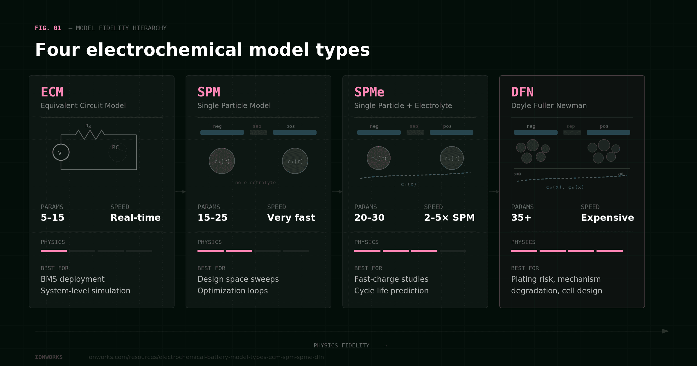
A full comparison of the electrochemical model hierarchy covers physics, parameterization, and compute cost across ECM, SPM, SPMe, and DFN.
When the form factor is large enough that in-plane heterogeneity matters — large-format pouch and prismatic cells, where tab placement concentrates current near terminals, where thermal hotspots build up at tabs or cell centers, and where electrode loading varies across the foot of the cell — even DFN's 1D-through-thickness resolution isn't enough. Aging is non-uniform across the cell area, not just across the electrode depth: hot regions degrade faster, regions near tabs see higher rates and more plating, and the cell ages from one corner inward. Pseudo-3D and full 3D electrochemical models resolve those gradients and couple them to the same mechanism submodels, so the why analysis carries through. In Ionworks, the same parameterized model extends from 1D SPMe or DFN to 3D without rewriting the parameter set.
What simulation reveals that bench cycling cannot
The variables that explain why are not directly measurable.
Anode potential. The threshold variable for plating. In a full cell, only terminal voltage is accessible; anode and cathode potentials require a reference electrode. Physics-based models compute anode potential at every time step.
Local SoC distribution. In a thick electrode at high C-rate, outer particles can be nearly full while inner particles are barely touched. This drives non-uniform mechanism rates. Invisible from terminal measurements.
Mode decomposition with mechanism attribution. A cell that has lost 20% capacity could have lost it primarily through LLI, primarily through LAM_ne or LAM_pe, or in combination — and the LLI could be from SEI growth, plating, or electrolyte depletion. A parameterized mechanism model decomposes capacity loss into mode and mechanism, informing which design lever to pull.
Extrapolation to new protocols. A cell tested at 1C charge for 500 cycles tells you how that cell ages at 1C. A mechanism model parameterized on that data extrapolates to 2C, to a different temperature profile, or to pulse charging — not perfectly, but far better than extrapolating an empirical curve, because it knows how each mechanism scales with conditions.
Formation protocol effects. The first cycles set the SEI baseline. Mechanism models simulate the downstream consequences of different formation choices without running multi-year aging studies for each.
The Ionworks workflow for degradation simulation
Ionworks supports all three approaches — empirical, per-mode empirical, mechanism-level — in one workflow, so the model can change as the question gets harder without changing the parameter set.
Parameterization handles the inverse problem: given full-cell OCV curves, rate capability, HPPC, and where available half-cell data and EIS, it fits the model parameters that best reproduce the measurements. Parameters are stored as validated, versioned parameterized models — not as loose scripts or spreadsheets. The parameter estimation guide covers the data requirements per model type.
With a parameterized model, teams run aging simulations across temperature, SoC window, voltage cutoffs, and C-rate. What is the capacity fade after 500 cycles at 35°C vs. 25°C? How does the rate change if the upper cutoff voltage is reduced from 4.2 V to 4.1 V? What is the plating risk at 2C charge across the temperature range? These studies take minutes to hours; the same exploration with physical testing takes months to years.
Degradation submodels attach mechanism-level processes to the simulation. LLI, LAM_ne, LAM_pe, and resistance growth come out as derived mode-level outputs alongside capacity and voltage curves, so the result includes both how the cell has degraded and why — which mechanism is dominant in each operating regime.
The same data infrastructure — cell instances, measurements, cycle metrics — feeds physics-based and ML workflows. Cycling data ingested from Maccor, Neware, Arbin, BioLogic, and Novonix cyclers flows directly into both. Every simulation is linked to the parameterized model and the protocol that generated it, so when a design changes the simulation history is preserved, and a new team member can reproduce any result from the record.
Choosing the right model for the question
| If you want to know... | Question type | Approach |
|---|---|---|
| Remaining useful life of cells in a deployed fleet | What | Empirical / ML on field data |
| Capacity at cycle 500 for a known chemistry under a known duty cycle | What | Single capacity-vs-cycle fit |
| Whether anode or cathode is limiting capacity fade | How | Per-mode empirical fits + dV/dQ on RPTs (LAM_ne vs. LAM_pe) |
How much of the loss is LLI vs. LAM_ne vs. LAM_pe | How | Per-mode empirical fits + dV/dQ on RPTs |
| Calendar aging rate across SoC × temperature (storage only, no cycling) | What | Arrhenius surface fit |
| Mixed duty cycle — storage composed with cycling (e.g., automotive parked 95% of the time, grid storage with intermittent dispatch) | Why | SPMe + SEI + plating submodels |
| Capacity fade and plating risk under a new fast-charge protocol | Why | SPMe + SEI + plating submodels |
Whether SEI or plating is driving LLI under fast charge | Why | SPMe with coupled SEI + plating submodels |
| Formation-protocol effect on long-term aging | Why | SPMe + SEI submodel with formation conditions |
| Spatial plating risk near the separator at 2C, low T | Why | DFN (anode-potential profile required) |
| Effect of electrode thickness, porosity, or graded architecture on aging | Why | DFN |
| Lifetime in a large-format pouch with in-plane gradients | Why | 3D electrochemical with degradation |
The model is not a one-time choice. As a design matures, the question moves from what (early screening) to how (mid-stage diagnosis) to why (most design and protocol decisions). A workflow that supports all three — and makes it easy to move between them — is more valuable than any single model.
Bench cycling answers the question that was asked. Simulation answers the questions that weren't.
Teams use Predict to run aging simulations across temperature, SoC window, and protocol space, with parameterized models built in Train. Book a demo to see degradation prediction running on your own cell data.
Frequently asked questions
Continue reading
Guide
Electrochemical battery model types compared: ECM, SPM, SPMe, and DFN
Guide
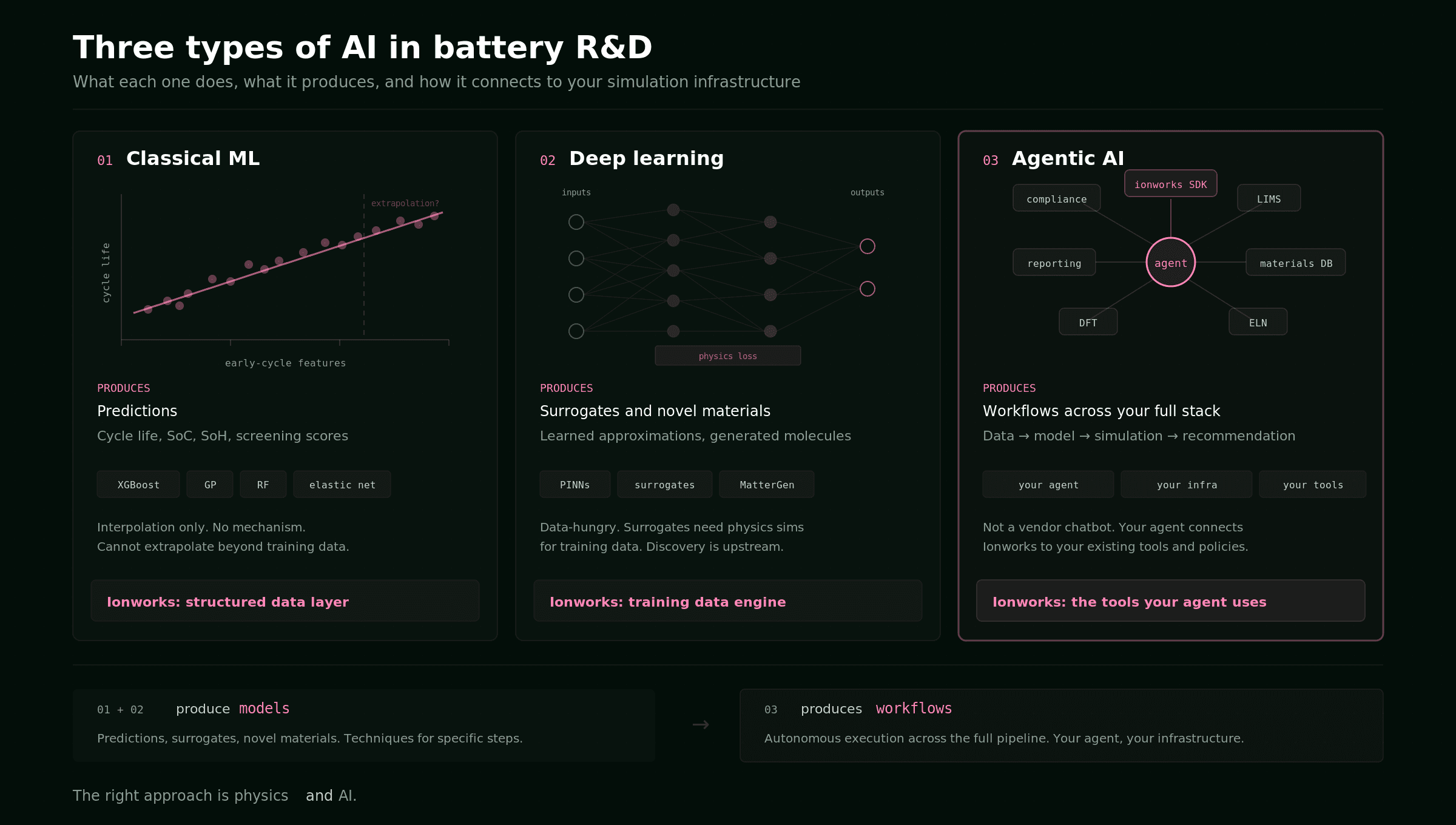
Three types of AI in battery R&D: classical ML, deep learning, and agentic workflows
Modeling
Battery Parameter Estimation for R&D Teams
Aging simulation